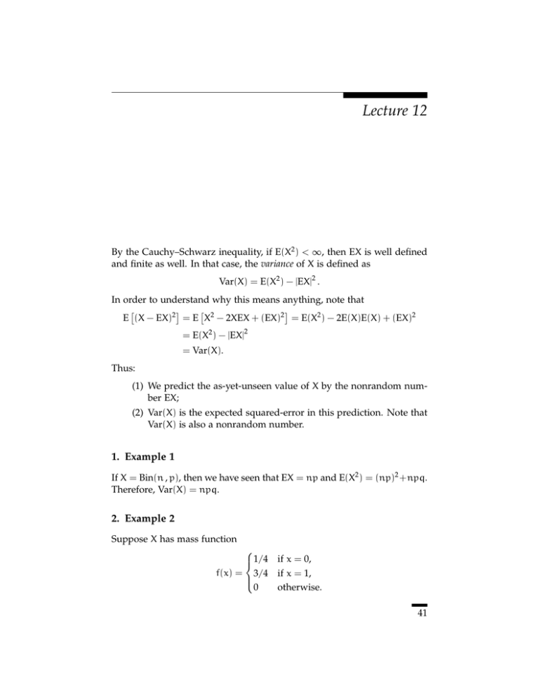
Lecture 12
By the Cauchy–Schwarz inequality, if E(X2 ) < ∞, then EX is well defined
and finite as well. In that case, the variance of X is defined as
Var(X) = E(X2 ) − |EX|2 .
In order to understand why this means anything, note that
"
!
"
!
E (X − EX)2 = E X2 − 2XEX + (EX)2 = E(X2 ) − 2E(X)E(X) + (EX)2
= E(X2 ) − |EX|2
= Var(X).
Thus:
(1) We predict the as-yet-unseen value of X by the nonrandom number EX;
(2) Var(X) is the expected squared-error in this prediction. Note that
Var(X) is also a nonrandom number.
1. Example 1
If X = Bin(n , p), then we have seen that EX = np and E(X2 ) = (np)2 +npq.
Therefore, Var(X) = npq.
2. Example 2
Suppose X has mass function


1/4 if x = 0,
f(x) = 3/4 if x = 1,


0
otherwise.
41
42
12
We saw in Lecture 11 that EX = 3/4. Now we compute the variance by
first calculating
#
$ #
$
1
3
3
2
2
2
E(X ) = 0 ×
+ 1 ×
= .
4
4
4
Thus,
Var(X) =
3
−
4
# $2
#
$
3
3
3
3
=
1−
= .
4
4
4
16
3. Example 3
Let n be a fixed positive integer, and X takes any of the values 1 , . . . , n with
equal probability. Then, f(x) = 1/n if x = 1, . . . , n; f(x) = 0, otherwise. Let
us calculate the first two “moments” of X.1 In this way, we obtain the mean
and the variance of X.
The first moment is the expectation, or the mean, and is
EX =
n
&
k
1
(n + 1)n
n+1
= ×
=
.
n
n
2
2
k=1
In order to compute E(X2 ) we need to know the algebraic identity:
n
&
k2 =
k=1
(2n + 1)(n + 1)n
.
6
(10)
This is proved by induction: For n = 1 it is elementary. Suppose it is true
for n − 1. Then write
n
&
2
k =
k=1
n−1
&
k=1
k2 + n2 =
(2(n − 1) + 1)(n − 1 + 1)(n − 1)
+ n2 ,
6
thanks to the induction hypothesis. Simplify to obtain
n
&
k2 =
k=1
(2n − 1)n(n − 1)
(2n − 1)(n2 − n)
+ n2 =
+ n2
6
6
2n3 − 3n2 + n 6n2
2n3 + 3n2 + n
n(2n2 + 3n + 1)
+
=
=
,
6
6
6
6
which easily yields (10).
=
Thus,
E(X2 ) =
n
&
k2
1
(2n + 1)(n + 1)n
(2n + 1)(n + 1)
= ×
=
.
n
n
6
6
k=1
1It may help to recall that the pth moment of X is E(Xp ).
43
5. Example 5
Therefore,
Var(X) =
(2n + 1)(n + 1)
−
6
#
n+1
2
$2
=
2n2 + 3n + 1 n2 + 2n + 1
−
6
4
4n2 + 6n + 2 3n2 + 6n + 3
−
12
12
2
n −1
=
.
12
=
4. Example 4
Suppose X = Poisson(λ). We saw in Lecture 10 that EX = λ. In order to
compute E(X2 ), we first compute E[X(X − 1)] and find that
E[X(X − 1)] =
∞
&
k(k − 1)
∞
e−λ λk & e−λ λk
=
k!
(k − 2)!
k=2
k=0
∞
&
e−λ λk−2
2
=λ
.
(k − 2)!
k=2
The sum is equal to one; change variables (j = k − 2) and recognize the jth
term as the probability that Poisson(λ) = j. Therefore,
E[X(X − 1)] = λ2 .
Because X(X − 1) = X2 − X, the left-hand side is E(X2 ) − EX = E(X2 ) − λ.
Therefore,
E(X2 ) = λ2 + λ.
It follows that
Var(X) = λ.
5. Example 5
Suppose f(x) = pqx−1 if x = 1, 2, . . .; and f(x) = 0 otherwise. This is the
Geometric(p) distribution. [The mass function for the first time to heads
for a p-coin; see Lecture 8.] We have seen already that EX = 1/p (Lecture
10). Let us find a new computation for this fact, and then go on and find
also the variance.
EX =
∞
&
kpqk−1 = p
k=1
d
=p
dq
%
∞
&
k=0
q
k
&
∞
&
kqk−1
k=1
d
=p
dq
#
1
1−q
$
=
p
1
= .
2
(1 − q)
p
44
12
Next we compute E(X2 ) by first finding
∞
&
∞
p&
E[X(X − 1)] =
k(k − 1)pq
=
k(k − 1)qk−2
q
k=1
k=1
%∞
&
#
$
2
&
1
d
p d2
k
= pq
q
=
dq2
q dq2 1 − q
k=0
#
$
d
1
2
2q
= pq
= pq
= 2.
2
3
dq (1 − q)
(1 − q)
p
k−1
Because E[X(X − 1)] = E(X2 ) − EX = E(X2 ) − (1/p), this proves that
E(X2 ) =
2q 1
2q + p
2−p
+ =
=
.
2
2
p
p
p
p2
Consequently,
2−p
1
1−p
q
− 2 =
= 2.
2
2
p
p
p
p
For a wholly different solution, see Example (13) on page 124 of your text.
Var(X) =