Lecture 22
1. Examples of continuous random variables
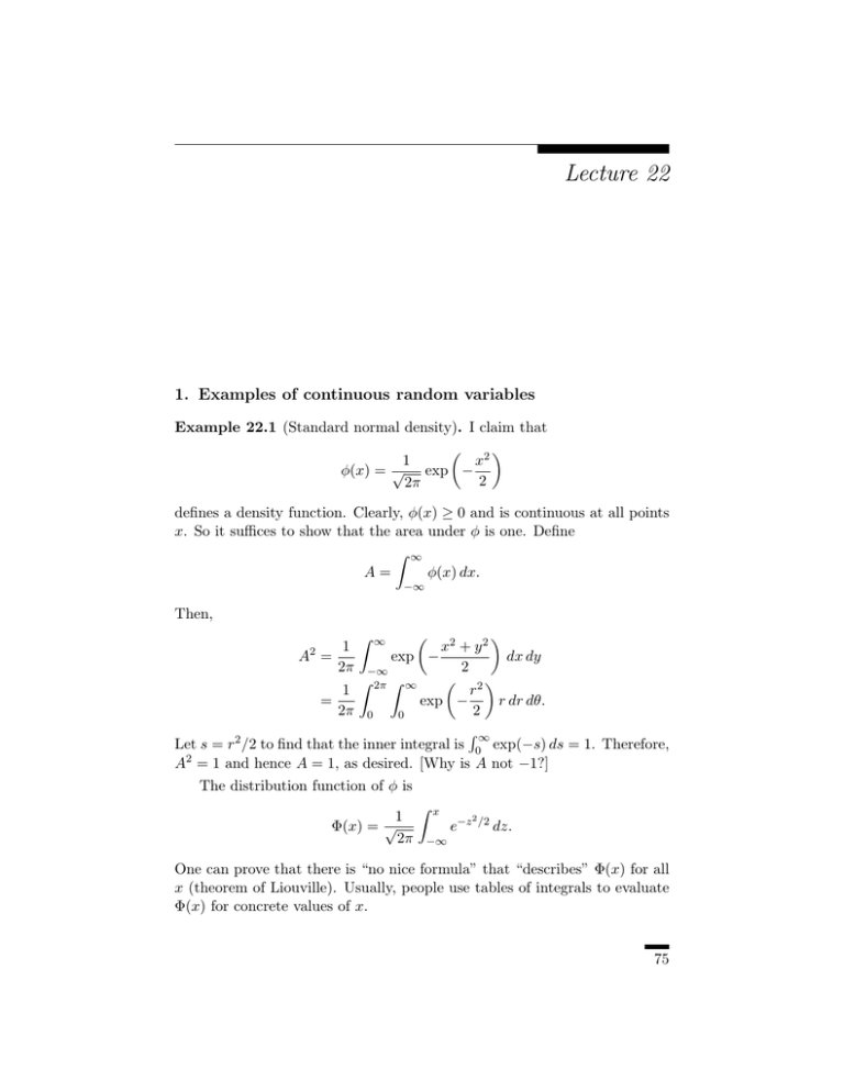
Example 22.1 (Standard normal density). I claim that
! 2"
1
x
φ(x) = √ exp −
2
2π
defines a density function. Clearly, φ(x) ≥ 0 and is continuous at all points
x. So it suffices to show that the area under φ is one. Define
# ∞
A=
φ(x) dx.
−∞
Then,
! 2
"
x + y2
exp −
dx dy
2
−∞
! 2"
# 2π # ∞
r
1
exp −
r dr dθ.
=
2π 0
2
0
$∞
Let s = r2 /2 to find that the inner integral is 0 exp(−s) ds = 1. Therefore,
A2 = 1 and hence A = 1, as desired. [Why is A not −1?]
A2 =
1
2π
#
∞
The distribution function of φ is
1
Φ(x) = √
2π
#
x
e−z
2 /2
dz.
−∞
One can prove that there is “no nice formula” that “describes” Φ(x) for all
x (theorem of Liouville). Usually, people use tables of integrals to evaluate
Φ(x) for concrete values of x.
75
76
22
Example 22.2 (Gamma densities). Choose and fix two numbers (parameters) α, λ > 0. The gamma density with parameters α and λ is the probability density function that is proportional to
%
xα−1 e−λx if x ≥ 0,
0
if x < 0.
Now,
#
∞
α−1 −λx
x
e
0
1
dx = α
λ
Define the gamma function as
# ∞
Γ(α) =
y α−1 e−y dy
#
∞
y α−1 e−y dy.
0
for all α > 0.
0
One can prove that there is “no nice formula” that “describes” Γ(α) for all α
(theorem of Liouville). Thus, the best we can do is to say that the following
is a Gamma density with parameters α, λ > 0:
 α
 λ xα−1 e−λx if x ≥ 0,
f (x) = Γ(α)

0
if x < 0.
$x
You can probably guess by now (and correctly!) that F (x) = −∞ f (y) dy
cannot be described by nice functions either. Nonetheless, let us finish by
making the observation that Γ(α) is computable for some reasonable values
of α > 0. The key to unraveling this remark is the following “reproducing
property”:
Γ(α + 1) = αΓ(α)
for all α > 0.
The proof uses integration by parts:
# ∞
Γ(α + 1) =
xα e−x dx
#0 ∞
=
u(x)v # (x) dx,
0
where u(x) = xα and v # (x) = e−x . Integration by parts states that1
#
#
#
uv = uv − v # u
for indefinite integrals.
1This follows immediately from integrating the product rule: (uv)! = u! v + uv ! .
(18)
77
2. Functions of a continuous random variable
Evidently, u# (x) = αxα−1 and v(x) = −e−x . Hence,
# ∞
Γ(α + 1) =
xα e−x dx
0
)∞ # ∞
)
= uv ) −
v#u
0
0
# ∞
*
+ )∞
α−1 −x )
= −αx
e
xα−1 e−x dx.
) +α
0
0
The first term is zero, and the$second (the integral) is αΓ(α), as claimed.
∞
Now, it easy to see that Γ(1) = 0 e−x dx = 1. Therefore, Γ(2) = 1×Γ(1) =
1, Γ(3) = 2 × Γ(2) = 2, . . . , and in general,
Γ(n + 1) = n!
for all integers n ≥ 0.
2. Functions of a continuous random variable
The basic problem: If Y = g(X), then how can we compute fY in terms of
fX ?
Example 22.3. Suppose X is uniform on (0 , 1), and Y = − ln X. Then,
we compute fY by first computing FY , and then using fY = FY# . Here are
the details:
FY (a) = P{Y ≤ a} = P {− ln X ≤ a} .
Now, − ln(x) is a decreasing function. Therefore, − ln(x) ≤ a if and only if
x ≥ e−a , and hence,
,
FY (a) = P X ≥ e−a = 1 − FX (e−a ).
Consequently,
d −a
(e ) = e−a fX (e−a ).
da
Now recall that fX (u) = 1 if 0 ≤ u ≤ 1 and fX (u) = 0 otherwise. Now e−a
is between zero and one if and only if a ≥ 0. Therefore,
%
1 if a ≥ 0,
fX (e−a ) =
0 if a < 0.
fY (a) = −fX (e−a )
It follows then that
%
e−a
fY (a) =
0
if a ≥ 0,
otherwise.
Thus, − ln X has an exponential density with parameter λ = 1. More generally, if λ > 0 is fixed, then −(1/λ) ln X has an exponential density with
parameter λ.
78
22
Example 22.4. Suppose X has density fX . Then let us find the density
function of Y = X 2 . Again, we seek to first compute FY . Now, for all a > 0,
, √
*√ +
* √ +
√ FY (a) = P{X 2 ≤ a} = P − a ≤ X ≤ a = FX
a − FX − a .
Differentiate [d/da] to find that
fY (a) =
√
√
fX ( a) + fX (− a)
√
2 a
On the other hand, fY (a) = 0 if a ≤ 0. For example, consider the case that
X is standard normal. Then,
 −a
 √e
if a > 0,
fX 2 (a) =
2πa

0
if a ≤ 0.
Or if X is Cauchy, then

 √ 1
fX 2 (a) = π a(1 + a)

0
if a > 0,
if a ≤ 0.
Example 22.5. Suppose µ ∈ R and σ > 0 are fixed constants, and define
Y = µ + σX. Find the density of Y in terms of that of X. Once again,
!
.
/
"
a−µ
a−µ
FY (a) = P {µ + σX ≤ a} = P X ≤
= FX
.
σ
σ
Therefore,
!
"
a−µ
1
.
fY (a) = fX
σ
σ
For example, if X is standard normal, then
!
"
1
(x − µ)2
fµ+σX (a) = √
exp −
.
2σ 2
2πσ 2
This is the socalled N (µ , σ 2 ) density.
Example 22.6. Suppose X is uniformly distributed on (0 , 1), and define

1

0 if 0 ≤ X < 3 ,
Y = 1 if 13 ≤ X < 23 ,


2 if 23 ≤ X < 1.
Then, Y is a discrete random variable with mass function,
%
1
if x = 0, 1, or 2,
fY (x) = 3
0 otherwise.
79
2. Functions of a continuous random variable
For instance, in order to compute fY (1) we note that
.
/ # 2/3
1
2
1
fY (1) = P
≤X<
=
fX (y) dy = .
1
23
4
3
3
3
1/3
≡1