Part 6: Genetic & Evolution
11/21/04
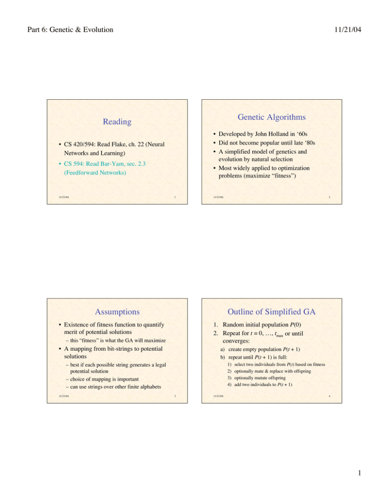
Genetic Algorithms
Reading
• Developed by John Holland in ‘60s
• Did not become popular until late ‘80s
• A simplified model of genetics and
evolution by natural selection
• Most widely applied to optimization
problems (maximize “fitness”)
• CS 420/594: Read Flake, ch. 22 (Neural
Networks and Learning)
• CS 594: Read Bar-Yam, sec. 2.3
(Feedforward Networks)
11/21/04
1
11/21/04
Assumptions
Outline of Simplified GA
• Existence of fitness function to quantify
merit of potential solutions
1. Random initial population P(0)
2. Repeat for t = 0, …, tmax or until
converges:
– this “fitness” is what the GA will maximize
• A mapping from bit-strings to potential
solutions
a) create empty population P(t + 1)
b) repeat until P(t + 1) is full:
– best if each possible string generates a legal
potential solution
– choice of mapping is important
– can use strings over other finite alphabets
11/21/04
2
1)
2)
3)
4)
3
11/21/04
select two individuals from P(t) based on fitness
optionally mate & replace with offspring
optionally mutate offspring
add two individuals to P(t + 1)
4
1
Part 6: Genetic & Evolution
11/21/04
Crossover: Biological Inspiration
Fitness-Biased Selection
• Want the more “fit” to be more likely to
reproduce
• Occurs during
meiosis, when haploid
gametes are formed
• Randomly mixes
genes from two
parents
• Creates genetic
variation in gametes
– always selecting the best
premature convergence
– probabilistic selection better exploration
• Roulette-wheel selection: probability relative fitness:
Pr{i mates} =
fi
n
j=1
fj
11/21/04
5
GAs: One-point Crossover
parents
11/21/04
(fig. from B&N Thes. Biol.)
11/21/04
6
GAs: Two-point Crossover
offspring
parents
7
11/21/04
offspring
8
2
Part 6: Genetic & Evolution
11/21/04
GAs: N-point Crossover
Mutation: Biological Inspiration
• Chromosome mutation • Gene mutation: alteration
of the DNA in a gene
– inspiration for mutation in
GAs
parents
• In typical GA each bit has
a low probability of
changing
• Some GAs models
rearrange bits
offspring
11/21/04
9
11/21/04
Example: GA for IPD
(fig. from B&N Thes. Biol.)
10
Typical Result
• Genetic strings encode strategy
– for first round
– based on self’s & opponent’s action on r
previous rounds
– hence 22r + 1 bits
convergence
• E.g., for r = 1:
opp. cooperated
opp. defected
we cooperated
first round
opp. defected
opp. cooperated
11/21/04
we defected
11
11/21/04
12
3
Part 6: Genetic & Evolution
11/21/04
The Red Queen Hypothesis
“Now, here, you see, it takes
all the running you can do,
to keep in the same place.”
— Through the Looking-Glass
and What Alice Found There
• Observation: a species
probability of extinction is independent of
time it has existed
• Hypothesis: species
continually adapt to
each other
• Extinction occurs with
insufficient variability
for further adaptation
11/21/04
13
...
...
a schema
110001
describes
many strings
11/21/04
*****0
**0*1*
11*0**
110*10
110010
11/21/04
14
• The schemata are the building blocks of
solutions
• We would like to know the average fitness
of all possible strings belonging to a schema
• We cannot, but the strings in a population
that belong to a schema give an estimate of
the fitness of that schema
• Each string in a population is giving
information about all the schemata to which
it belongs (implicit parallelism)
A schema is a description of certain patterns
of bits in a genetic string
111010
The Schema Theorem
The Fitness of Schemata
Schemata
110000
Why Does the GA Work?
110010
a string
belongs to
many schemata
15
11/21/04
16
4
Part 6: Genetic & Evolution
11/21/04
Effect of Selection
Exponential Growth
Let n = size of population
Let m( S,t ) = number of instances of schema S at time t
String i gets picked with probability
fi
j
fj
• Suppose f(S) = fav (1 + c)
Let f ( S ) = avg fitness of instances of S at time t
So expected m( S,t + 1) = m( S,t ) n Since f av =
j
n
fj
• Then m(S, t) = m(S, 0) (1 + c)t
f ( S)
, m( S,t + 1) = m( S,t )
fj
j
• That is, exponential growth in aboveaverage schemata
f ( S)
f av
11/21/04
17
Effect of Crossover
• We have discovered:
m(S, t+1) = m(S, t) f(S) / fav
**1 … 0***
||
11/21/04
Selection & Crossover Together
• Let = length of genetic strings
• Let (S) = defining length of schema S
• Probability {crossover destroys S}:
pd (S) / ( – 1)
• Let pc = probability of crossover
• Probability schema survives:
ps 1 pc
11/21/04
18
m( S,t + 1) m( S,t )
f (S) (S ) 1 pc
f av 1
( S)
1
19
11/21/04
20
5
Part 6: Genetic & Evolution
11/21/04
Effect of Mutation
Schema Theorem:
“Fundamental Theorem of GAs”
• Let pm = probability of mutation
• So 1 – pm = probability an allele survives
• Let o(S) = number of fixed positions in S
m( S,t + 1) m( S,t )
• The probability they all survive is
(1 – pm)o(S)
f (S) (S )
o( S ) pm 1 pc
f av 1
• If pm << 1, (1 – pm)o(S) 1 – o(S) pm
11/21/04
21
11/21/04
22
The Bandit Problem
• Two-armed bandit:
– random payoffs with (unknown) means m1, m2
and variances 1, 2
– optimal strategy: allocate exponentially greater
number of trials to apparently better lever
Goldberg’s Analysis of
Competent & Efficient GAs
• k-armed bandit: similar analysis applies
• Analogous to allocation of population to
schemata
• Suggests GA may allocate trials optimally
11/21/04
23
11/21/04
24
6
Part 6: Genetic & Evolution
11/21/04
Race Between Selection &
Innovation: Takeover Time
Paradox of GAs
• Individually uninteresting operators:
– selection, recombination, mutation
• Takeover time t* = average time for most fit
to take over population
• Transaction selection: top 1/s replaced by s
copies
• Selection + mutation continual
improvement
• Selection + recombination innovation
– generation vs.evaluation
s quantifies selective pressure
• Fundamental intuition of GAs: the three
work well together
11/21/04
• Estimate t* ln n / ln s
25
11/21/04
Innovation Time
Steady State Innovation
• Bad: t* < ti
• Innovation time ti = average time to get a
better individual through crossover &
mutation
• Let pi = probability a single crossover
produces a better individual
• Number of individuals undergoing
crossover = pc n
• Probability of improvement = pi pc n
• Estimate: ti 1 / (pc pi n)
11/21/04
26
– because once you have takeover, crossover
does no good
• Good: ti < t*
– because each time a better individual is
produced, the t* clock resets
– steady state innovation
• Innovation number:
t*
n ln n
Iv = = pc pi
>1
ln s
ti
27
11/21/04
28
7
Part 6: Genetic & Evolution
11/21/04
Other Algorithms Inspired by
Genetics and Evolution
Feasible Region
pc
successful
genetic algorithm
• Evolutionary Programming
cross-competition
boundary
drift boundary
crossover probability
schema theorem boundary
– natural representation, no crossover,time-varying
continuous mutation
• Evolutionary Strategies
– similar, but with a kind of recombination
• Genetic Programming
– like GA, but program trees instead of strings
• Classifier Systems
mixing boundary
– GA + rules + bids/payments
selection pressure
11/21/04
ln s
29
• and many variants & combinations…
11/21/04
30
Additional Bibliography
1. Goldberg, D.E. The Design of Innovation:
Lessons from and for Competent Genetic
Algorithms. Kluwer, 2002.
2. Milner, R. The Encyclopedia of
Evolution. Facts on File, 1990.
11/21/04
31
8