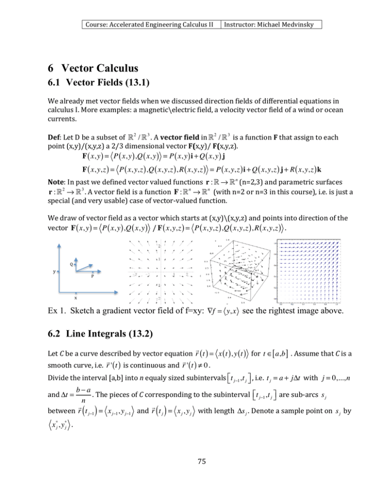
Course: Accelerated Engineering Calculus II Instructor: Michael Medvinsky 6 Vector Calculus
6.1 Vector Fields (13.1)
We already met vector fields when we discussed direction fields of differential equations in calculus I. More examples: a magnetic\electric field, a velocity vector field of a wind or ocean currents. Def: Let D be a subset of  2 /  3 . A vector field in  2 /  3 is a function F that assign to each point (x,y)/(x,y,z) a 2/3 dimensional vector F(x,y)/ F(x,y,z). F ( x, y ) = P ( x, y ) ,Q ( x, y ) = P ( x, y ) i + Q ( x, y ) j
F ( x, y, z ) = P ( x, y, z ) ,Q ( x, y, z ) , R ( x, y, z ) = P ( x, y, z ) i + Q ( x, y, z ) j + R ( x, y, z ) k
Note: In past we defined vector valued functions r :  →  n (n=2,3) and parametric surfaces r :  2 →  3 . A vector field is a function F :  n →  n (with n=2 or n=3 in this course), i.e. is just a special (and very usable) case of vector-­‐valued function. We draw of vector field as a vector which starts at (x,y)\(x,y,z) and points into direction of the vector F ( x, y ) = P ( x, y ) ,Q ( x, y ) / F ( x, y, z ) = P ( x, y, z ) ,Q ( x, y, z ) , R ( x, y, z ) . Q y P x Ex 1. Sketch a gradient vector field of f=xy: ∇f = y, x see the rightest image above.
6.2 Line Integrals (13.2)

Let C be a curve described by vector equation r ( t ) = x ( t ) , y ( t ) for t ∈[ a,b ] . Assume that C is a 

smooth curve, i.e. r ' ( t ) is continuous and r ' ( t ) ≠ 0 . Divide the interval [a,b] into n equaly sized subintervals ⎡⎣t j−1 ,t j ⎤⎦ , i.e. t j = a + jΔt with j = 0,...,n b−a
. The pieces of C corresponding to the subinterval ⎡⎣t j−1 ,t j ⎤⎦ are sub-­‐arcs s j n


between r t j−1 = x j−1 , y j−1 and r t j = x j , y j with length Δs j . Denote a sample point on s j by
and Δt =
( )
( )
x *j , y*j . 75 Course: Accelerated Engineering Calculus II Instructor: Michael Medvinsky Consider that a function f(x,y) is defined on all points of the curve C. The following sum looks n
(
)
very similar to Reimann sum: ∑ f x *j , y*j Δs j j=1


Def: If f is defined on a smooth curve C given by r ( t ) = x ( t ) , y ( t ) or r ( t ) = x ( t ) , y ( t ) , z ( t ) , then the line\contour\path\curve integral is defined by: (
n
)
n
*
*
f ( x, y ) ds = 
∫ f ( x, y ) ds = lim ∑ f x j , y j Δs j
∫
C
n→∞
C
j=1
(
)
*
* *
∫ f ( x, y, z ) ds = lim ∑ f x j , y j , z j Δs j or
n→∞
C
j=1
if the limit exists. Reminder: The length of the curve C is given by 2
b
2
b
∫ f ( x, y ) ds = ∫
C
a
2
2
⎛ dx ⎞ ⎛ dy ⎞ ⎛ dz ⎞
L = ∫ ⎜ ⎟ + ⎜ ⎟ + ⎜ ⎟ dt ⎝ dt ⎠ ⎝ dt ⎠ ⎝ dt ⎠
a
or
2
b
2
ds
⎛ dx ⎞ ⎛ dy ⎞
f ( x ( t ) , y ( t )) dt = ∫ f ( x ( t ) , y ( t )) ⎜ ⎟ + ⎜ ⎟ dt
⎝ dt ⎠ ⎝ dt ⎠
dt
a
b
∫ f ( x, y, z ) ds = ∫
C
2
b
⎛ dx ⎞ ⎛ dy ⎞
L = ∫ ⎜ ⎟ + ⎜ ⎟ dt
⎝ dt ⎠ ⎝ dt ⎠
a
Thm: If f is continues then a
or
2
b
2
2
ds
⎛ dx ⎞ ⎛ dy ⎞ ⎛ dz ⎞
f ( x ( t ) , y ( t ) , z ( t )) dt = ∫ f ( x ( t ) , y ( t ) , z ( t )) ⎜ ⎟ + ⎜ ⎟ + ⎜ ⎟ dt
⎝ dt ⎠ ⎝ dt ⎠ ⎝ dt ⎠
dt
a
regardless of the parameterization as long as the curve traversed exactly once between a and b , i.e. it doesn’t wind circles. b
b



Note: One can rewrite the formulas above as L = ∫ r ' ( t ) dt and 
∫ f ( x, y, z ) ds = ∫ f ( r (t )) r '(t ) dt a
C
a

Ex 2. Let C be a curve defined by r (t) = 2 cost,2sint , 0 ≤ t ≤ π
∫x
C
π
2
( −2sint ) + ( 2 cost )
y ds = ∫ 4 cos t ⋅ 2sint ⋅
2
2
0
2
π
dt = 16 ∫ cos t ⋅sint dt
2
0
u=cost
du=− sintdt
=
1
16 ∫ u 2 du =
t=0⇒u=1
t=π ⇒u=−1
−1

Ex 3. Let C be a curve defined by r (t) = −t, 3 + 3t,6 + 5t , − 1 ≤ t ≤ 0
0
32
3
0
35 35
2
C
−1
−1
Def: Given C j ,1 ≤ j ≤ n are smooth curves the curve C = C1 ∪ C2 ∪ ...∪ Cn called piecewise smooth. ∫ (x + 2y + 4z)ds = ∫ ( −t + 6 + 6t + 24 + 20t )
1+ 9 + 25 dt = 35 ∫ 25t + 30 dt =
n


f
r
t
ds
=
Thm: For a piecewise smooth C = C1 ∪ C2 ∪ ...∪ Cn we have 
(
)
(
)
∑ ∫ f ( r (t )) ds . ∫
j=1 C j
C

C1 : r (t) =
Ex 4.
∫
C1 ∪C2
∫(

C2 : r (t) = 1,2,−5t , − 1 ≤ t ≤ 0
8t, 4t,5t , 0 ≤ t ≤ 1,
x + y + z ds = 
∫ x + y + z ds + ∫ x + y + z ds =
C1
1
8t + 4t + 5t
0
)
C2
0
8 + 16 + 25 dt + ∫ (1+ 2 − 5t ) 0 2 + 0 2 + 25 dt =
−1
(
)
1
0
7 9+ 8
⎛
t2
t2 ⎞
25
7 9 + 8 ∫ t dt + 5 ∫ 3 − 5t dt = 7 9 + 8
+ 5 ⎜ 3t − 5 ⎟ =
+ 35 +
20
2 ⎠ −1
2
2
⎝
0
−1
(
)
1
0
(
)
76