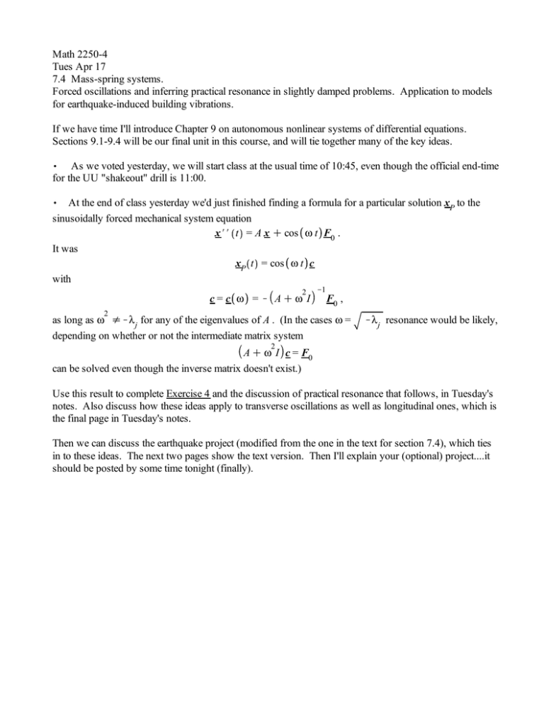
Math 2250-4
Tues Apr 17
7.4 Mass-spring systems.
Forced oscillations and inferring practical resonance in slightly damped problems. Application to models
for earthquake-induced building vibrations.
If we have time I'll introduce Chapter 9 on autonomous nonlinear systems of differential equations.
Sections 9.1-9.4 will be our final unit in this course, and will tie together many of the key ideas.
, As we voted yesterday, we will start class at the usual time of 10:45, even though the official end-time
for the UU "shakeout" drill is 11:00.
, At the end of class yesterday we'd just finished finding a formula for a particular solution xP to the
sinusoidally forced mechanical system equation
x## t = A x C cos w t F0 .
It was
xP t = cos w t c
with
2
c = c w = K ACw I
2
K1
F0 ,
as long as w sKl j for any of the eigenvalues of A . (In the cases w =
depending on whether or not the intermediate matrix system
Kl j resonance would be likely,
2
A C w I c = F0
can be solved even though the inverse matrix doesn't exist.)
Use this result to complete Exercise 4 and the discussion of practical resonance that follows, in Tuesday's
notes. Also discuss how these ideas apply to transverse oscillations as well as longitudinal ones, which is
the final page in Tuesday's notes.
Then we can discuss the earthquake project (modified from the one in the text for section 7.4), which ties
in to these ideas. The next two pages show the text version. Then I'll explain your (optional) project....it
should be posted by some time tonight (finally).
step 1) understand the model above. (Note, the Maple commands are out of date.)
step 2) understand the table below:
step 3) understand the inhomogeneous DE below in (2), and why the forcing term has the claimed form.
step 4) understand the practical resonance graph, figure 7.4.18, and how it relates to the natural periods in
Figure 7.4.17.
In your Maple project you will be working with a 4-story building. In addition to finding the 4 natural
frequencies and periods, and a practical resonance graph analogous to 7.4.18, you will describe the four
fundamental modes of vibration. You may use Maple, Matlab, Mathematica, Wolfram alpha - whatever
software you prefer. You will upload your results to CANVAS.
Here is a demonstration video of what happens for buildings with one, two, or three stories. The driving
frequency is steadily increased, and various modes are excited (but not all of them).
http://www.youtube.com/watch?v=M_x2jOKAhZM
modeling the 3 story building, as in the youtube video:
The ground is moving sinusoidally with amplitude E ,
x0 t = E cos w t
and acceleration
2
x0 ## t =KE w cos w t
the accelerations of the three massive floors (the top one is the roof) above ground, relative to the frame of
the moving ground are therefore given by
x1 ## t
x1 t
K2 1 0
1
x2 ## t
x3 ## t
=
k
m
1
x2 t
1 K1
x3 t
1 K2
0
C Ew2 cos w t
1
.
1
Note the K1 value in the last diagonal entry. This is because x3 t is measuring displacements for the top
floor (roof), which has nothing above it.
Exercise i) do you understand how that inhomogeneous system of DE's arises?
k
= 1 . Maple does not realize the eigenvalues are real
m
numbers, and so several extra commands are needed to extract clear information.
> with LinearAlgebra :
> A d Matrix 3, 3, K2, 1.0, 0, 1,K2, 1, 0, 1,K1 ;
# I used one decimal value so Maple would evaluate in floating point
Eigenvectors A ; # execute these commands to see the mess.
> Digits d 5 : # 5 digits should be fine, for one thing.
clean up the mess:
> eigendata d Eigenvectors A :
eigendata 1 : #eigenvalues
eigendata 2 : #corresponding eigenvectors
lambdas d map R, eigendata 1 : # get rid of the 0 i's by taking real part.
omegas d map sqrt,Klambdas ; # natural angular frequencies
2$evalf Pi
f d x/
:
x
periods d map f, omegas ; #natural periods
vectors1 d map R, eigendata 2 : # eigenvectors for fundamental modes
vectors d map evalf, vectors1 ; # get the digits down to 5
Here is eigendata for the unscaled matrix
1.8019
omegas :=
1.2470
0.44504
3.4870
periods :=
5.0386
14.118
vectors :=
0.59101
0.73698
0.32799
K0.73698
0.32799
0.59101
0.32799
(1)
K0.59101 0.73698
>
k
= 1)
m
. In the youtube video the first mode to appear is the slow and dangerous "sloshing mode", where all three
floors oscillate in phase, with amplitude ratios 33 : 59 : 74 from the first to the third floor. What's the
second mode that gets excited? The third mode?
Exercise ii) Interpret the data above, in terms of the natural modes for the shaking building (when
Exercise iii) Could you modify the matrix algebra, and then the commands in yesterday's notes, to create
practical resonance graphs as we did there?
Introduction to Chapter 9: Autonomous first order systems of differential equations
The general system of two first order differential equations for x t , y t can be written as
x# t = F x t , y t , t
y# t = G x t , y t , t
which we abbreviate as usual, by writing
x#= F x, y, t
y#= G x, y, t .
If the rates of change F, G only depend on the values of x t , y t but not on t , i.e.
x#= F x, y
y#= G x, y
then the system is called autonomous. Autonomous systems are the focus of Chapter 9.
Constant solutions to autonomous systems are called equilibrium solutions. Thus, equilibrium solutions
x t h x), y t h y * will correspond to solutions x), y) T to the nonlinear algebraic system
F x, y = 0
G x, y = 0
Exercise 1) Consider the "competing species" model from 9.2, shown below. For example and in
appropriate units, x t might be a squirrel population and y t might be a rabbit population, competing on
the same island sanctuary.
x# t = 14 x K 2 x2 K x y
y# t = 16 y K 2 y2 K x y .
1a) Notice that if either population is missing, the other population satisfies a logistic DE. Discuss how
the signs of third terms on the right sides of these DEs indicate that the populations are competing with
each other (rather than, for example, acting in symbiosis, or so that one of them is a predator of the other).
1b) Find the four equilibrium solutions to this competition model, algebraically.
Equilibrium solutions x), y)
T
to first order autonomous systems
x#= F x, y
y#= G x, y
are called stable if solutions to IVPs starting close (enough) to x), y) T stay as close as desired.
, Equilibrium solutions are unstable if they are not stable.
, Equilibirum solutions x), y) T are called asymptotically stable if they are stable and furthermore, IVP
,
solutions that start close enough to x), y)
T
converge to x), y)
T
as t/N .
1c) Discuss the pplane phase portrait below for the competition model on the previous page. Discuss the
sorts of stability/instability exhibited by the four equilibrium solutions.
1d) Where are the two phase diagrams from Chapter 2, for the logistic behavior when there is only one
population, in the phase portrait below?
1e) If both initial populations are positive, what do you expect their limiting populations will be?