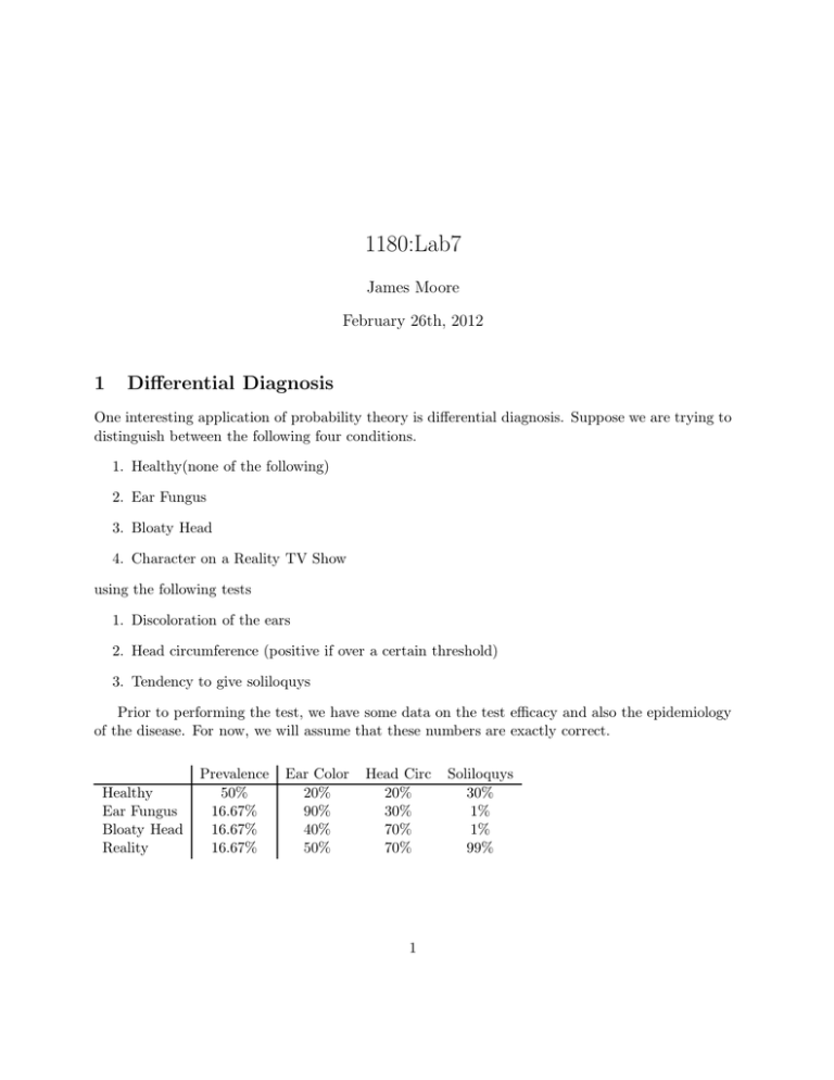
1180:Lab7
James Moore
February 26th, 2012
1
Differential Diagnosis
One interesting application of probability theory is differential diagnosis. Suppose we are trying to
distinguish between the following four conditions.
1. Healthy(none of the following)
2. Ear Fungus
3. Bloaty Head
4. Character on a Reality TV Show
using the following tests
1. Discoloration of the ears
2. Head circumference (positive if over a certain threshold)
3. Tendency to give soliloquys
Prior to performing the test, we have some data on the test efficacy and also the epidemiology
of the disease. For now, we will assume that these numbers are exactly correct.
Healthy
Ear Fungus
Bloaty Head
Reality
Prevalence
50%
16.67%
16.67%
16.67%
Ear Color
20%
90%
40%
50%
Head Circ
20%
30%
70%
70%
1
Soliloquys
30%
1%
1%
99%
2
Questions
Use probability theory to find the following.
1. The probability that someone tests positive for ear discoloration.
2. The probability that someone tests positive for large head circumference.
3. ...for soliloquys.
4. Suppose that has discolored ears. Use conditional probability to find the probability that
they are:Healthy, suffering from ear fungus, have a bloaty head or are a Reality TV Star.
3
Simulating Lots of Tests
To gain some insight into how these tests work together we will simulate a population of 10000
people, run each test on them and then examine the resulting data.
Disease_Names=c("Healthy","Ear Fungus","Bloaty Head Disease","Reality TV Contestant")
Incidence=c(50,16.67,16.67,16.67)
N=10000 #Number of Patients
#Positive for Test A (Ear Color Test)
A_pos=c(.2,.9,.4,.5)
#Positive for Test B (Measure Head Circumference)
B_pos=c(.2,.3,.7,.7)
#Positive for Test C (Random Soliloquys)
C_pos=c(.3,.01,.01,.99)
#Generate Diseases
D_Numbers=sample(1:4,N,prob=Incidence,replace=T)
#Match Numbers to Hilarious Names
Diseases=Disease_Names[D_Numbers]
#Simulate Tests
A_result=rbinom(N,size=1,prob=A_pos[D_Numbers])
B_result=rbinom(N,size=1,prob=B_pos[D_Numbers])
C_result=rbinom(N,size=1,prob=C_pos[D_Numbers])
2
#Put in a data frame
Patients=data.frame(Diseases,A_result,B_result,C_result)
The variable ‘Patients’ contains all of our data. Trying to read through it would be a waste of
time. Instead we can count the numbers of people with weird looking ears.
> sum(Patients$A_result)
[1] 3983
Then we can get a breakdown of the conditions of all those people.
> summary(Patients[A_result==1,"Diseases"])
Bloaty Head Disease
Ear Fungus
665
1483
Reality TV Contestant
853
Healthy
982
For my data, I see that 37% (1483/3983) of people who test positive for ”Ear Discoloration” actually
have Ear Fungus. This number will be different for you. Next we can look at all the people who
have Ear Fungus but don’t give soliloquys. First here’s the breakdown.
> summary(Patients[A_result==1&C_result==0,"Diseases"])
Bloaty Head Disease
Ear Fungus
655
1469
Reality TV Contestant
7
Healthy
696
Then we can sum this list to get the total number of people positive for one test not the other.
> sum(summary(Patients[A_result==1&C_result==0,"Diseases"]))
[1] 2827
With both test results, the odds have improved to 52% (1469/2827)
4
More Questions!
1. Check all your answers to the first part using the simulation data. Give your prediction along
with what the data tells you both as raw numbers and a percentage.
2. We have three tests meaning there are 8 possible outcomes. (All Negative, All positive, Only
one test positive (3), Only one test negative(3)). For each case, give the most likely condition
(healthy, ear fungus,etc) and how likely it is to be that disease. (There’s another page!)
3
3. Add one new test and one new disease to the list. Adjust the prevalence so they still add up
to one 100% and make the test outcomes whatever you want (can’t be less than 0 or more
than 100%), but be sure to provide them. In addition, modify the code and include it in your
final document.
Run a simulation and then pick one hypothetical series of test outcomes. Can you figure out
what the patient has?
4