Calculus for Biologists Lab
Math 1180-002
Spring 2012
Lab #4 - Stochastic Population Growth
Report due date: Tuesday, February 14, 2012 at 9 a.m.
Goal: To explore similarities and differences between models of population growth based on production and
immigration. You will observe what it means to have a population or other quantity determined by probabilities
and stochastic behavior.
? Create a new script, either in R (laptop) or with a text editor (Linux computers).
‘for’ loop fun
for loops are used for a variety of things. In this lab, we will use them to modify a population’s size over time
based on its size at previous times. You may remember that you implemented loops to simulate discrete-time
systems last semester. The following code defines a population’s size in discrete time points based on the updating
function f (b) = rb and the corresponding discrete equation
bt+1 = f (bt ) = rbt .
Please pay attention to the comments, as you will be expected to modify this loop later in the lab.
## Preliminaries
N = 50
## total number of time steps
r = 1.1
## define growth rate r
init.pop = 1
## define initial population size
## Set up a list, b,
b = matrix(init.pop,
N+1,
1)
to
##
##
##
save population sizes at each time (can write this in 1 line too)
every spot in b (arbitrarily) starts with init.pop things
there are N+1 total spots (times), including t = 0
we only care about 1 population
## Now start the 'for' loop
for (j in 1:N){
## index things with j, ranging from time 1 to time N
b[j+1, ] = r*b[j, ] ## update current pop. using previous size b[j] and growth rate
}
## end when j = N
## Now plot the solution
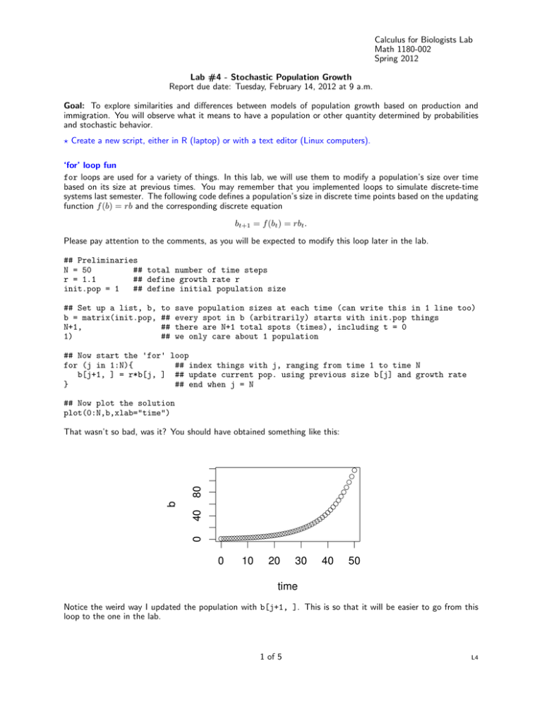
plot(0:N,b,xlab="time")
0
40
b
80
That wasn’t so bad, was it? You should have obtained something like this:
0
10
20
30
40
50
time
Notice the weird way I updated the population with b[j+1, ]. This is so that it will be easier to go from this
loop to the one in the lab.
1 of 5
L4
Simulating stochastic growth: production
Let’s say we have some population of things, bacteria, people, etc. And let’s say that the average growth rate
of the population is 1.1. There are instances when the growth rate is smaller, others when it is larger. How do
we assess the overall behavior of the population given that the growth rate can change randomly? This is where
stochastic growth comes in. The first type we will consider is with respect to production. An individual in the
population reproduces at some randomly chosen rate. Because it’s our model, we can also specify a range for
these growth rates. So, let’s say we start with a single entity in the population, and we decide that the average
growth rate will be 1.1, but the precise rates we use can range between 0.8 and 1.4. Can you predict what will
happen to the population over the long run?
To explore this question, we will simulate multiple populations according to the discrete-time equation
bt+1 = rt bt ,
(1)
where it’s assumed that growth rate rt does not have to be the same for all time points we use. In fact, we
are going to randomly pick rt . To do this, we need to know how to generate random numbers in R. The
command runif(how_many_you_want, min=min_value, max=max_value) picks how ever many numbers we
want, between a minimum and maximum value, all chosen with equal probability. Let’s say we want 10 numbers
ranging between 100 and 105.
runif(10, min=100, max=105)
Now execute this line again; you will very likely get completely different numbers from the first set.
We will not just simulate a single population. What if we wanted to look at the behavior of ten different
populations over time? To start, we have to define some preliminary values.
N = 50
n.sim = 10
## number of time points
## number of populations
init.pop = 1 ## initial population size
Now, we turn to the weird notation from the earlier loop example. In order to track multiple populations, we
need some way of storing the information. To do this, you’ll use the matrix command, which will essentially
function as a table to put values in. If we are interested in both the population sizes AND the corresponding rates
at various time points, we can set up two empty tables into which we can store our numbers. b will denote the
population size and r the growth rate.
b = matrix(0,N+1,n.sim)
r = matrix(0,N+1,n.sim)
This tells R to create a table of all zeros with N + 1 rows (the time points) and n.sim columns (the populations).
To access these values, we use the notation b[R,C]. This will show us the number in row R and column C of
table b.
Detour
To see an example, execute the following lines.
## execute these first
test.matrix = matrix(1:9,3,3)
test.matrix
## now do this one
test.matrix[3,2]
## and now these
test.matrix[3,2] = 200
test.matrix
Back to business
Now that you have a better understanding of how we store our results, we are ready to simulate!
First, initialize each population using the value we defined earlier. This amounts to setting each number in the
first row of b (spanning all columns) to init.pop.
b[1, ] = init.pop
2 of 5
L4
Notice the empty space between the comma and end bracket. This tells R to place the designated value in each
spot for row 1.
Second, determine the growth rate at time zero by choosing n.sim random numbers ranging from 0.8 to 1.4.
(What’s the average of these numbers?) Unlike in the previous line of code, none of these numbers should be the
same, but we can still tell R to assign one number to each spot in row 1 of our r table.
r[1, ] = runif(n.sim,min=0.8,max=1.4)
Finally, you can implement the for loop (fun!). I will outline what you need to do, but it is your job to create
the code to do it. The table format allows us to simulate changes in all n.sim populations simultaneously.
• Execute the loop for times between 1 and N .
• Use the form bt+1 = rt bt as your updating function inside the loop, which is very similar to the example at
the start of the lab.
• Note that the major difference is in r, which now also changes with each time point. So, update rt+1 by
choosing random numbers in the exact same way as above.
A natural next step is to plot the results. Before we get to this, though, it’s often useful to have something to
which we can compare them. So, think back to last semester, summon your knowledge of discrete-time systems
and solve (with pencil, paper ... and perhaps an eraser too) the deterministic equation
bt+1 = rbt ,
b0 = 1,
with r = 1.1. Think about why it makes sense to do this, based on the range of rt values used in the simulations.
Execute the following code, typing in the solution you obtained in the right-hand side of B, replacing any t you
have with time.
time = seq(0,N,by=0.1)
B = ## your solution goes here
And, plot:
colors = rainbow(n.sim)
matplot(0:N,b, col=colors, type="o", pch = 1:n.sim, ylim=c(0,max(b,B)),ann=F)
lines(time,B,type="l",lwd=2) ## plot deterministic case
title(main="Stochastic population growth: production",xlab="Time",ylab="Population")
The solution you determined should appear as the thicker black line. Judging from the results of your n.sim
simulations, the placement of the black line should make sense. If it doesn’t, you may need to check your math
and/or your loop.
?
What are some similarities and differences you see among the dynamics
and long term behavior of each population in this stochastic production
model? Be thorough in your description.
?
Pick a number between 1 and n.sim, type it into the code below, and execute. We’ll come back to this.
my.pop.growth = ## your number goes here
b1 = b[ ,my.pop.growth]
r1 = r[ ,my.pop.growth]
Simulating stochastic growth: immigration
You just saw an example of a series of populations that rely on reproduction for growth. But, what if you have
some area, and every now and then – each year, say – there’s some probability p that exactly three individuals
(or none at all) will immigrate? The corresponding stochastic formulation would be
bt + 3,
with probability p,
bt+1 =
(2)
bt ,
with probability 1 − p.
Set init.pop to zero for this model. Let q be the immigration term, which equals 3 with probability p and 0
3 of 5
L4
with probability 1 − p. We will define the function immigration to describe this situation. In doing so, we need
to make use of the following command:
sample(what_to_sample,how_many_you_want,replace=TRUE/FALSE, prob=probabilities). Executing the
line
sample(c(100,500),10,replace=FALSE,prob=c(0.2,0.8))
should leave you with an error. This is because the option replace=FALSE tells R that once you pick both
numbers, you have nothing left to choose from. Since we want ten numbers, R doesn’t know what to do. Change
FALSE to TRUE and re-execute the line. You should now have a list of ten numbers that only includes 100 and
500 as its elements. Count how many 100s you have and how many 500s. This difference is attributed to the
probability list c(0.2,0.8), which tells R to choose 100 with probability 0.2 and 500 with probability 0.8. So,
the result is that you get more 500s in your list than 100s.
Now, define the function immigration(p) in R that samples n.sim numbers of 0s and 3s with probability p of
getting a 3.
immigration = function(p) ## fill in the rest
Test your work by evaluating immigration(0.2). Is the result what you expected? If so, continue.
As with rt from before, we will keep track of different values of q over time. So we’ll define the empty tables b
and q, initialize them, and run the simulation for the same N time points and n.sim number of populations as
before.
b = matrix(0,N+1,n.sim)
q = matrix(0,N+1,n.sim)
b[1, ] = init.pop
q[1, ] = immigration(0.5)
Now execute an appropriately modified loop. You can check that you’ve done this correctly with the upcoming
plot commands. Because it’s useful to compare simulations to mathematical results, we will define the solution
to the representative deterministic equation.
time = seq(0,N,by=0.1)
B = 1.5*time
Don’t just take this as fact! Explain why this expression for B
represents the stochastic model. Use some investigative techniques if
you have to.
?
?
Plot these results:
colors = rainbow(n.sim)
matplot(0:N,b, col=colors, pch=1: n.sim, type="o",ylim=c(0,max(b)),ann=F)
lines(time,B,type="l",lwd=2)
title(main="Stochastic population growth: immigration",xlab="Time",ylab="Population")
Remember, if the deterministic and stochastic representations don’t seem to correspond with each other at all,
you will need to correct your loop.
?
What are some similarities and differences you see among the dynamics
and long term behavior of each population in this stochastic
immigration model? Be thorough in your description.
?
Pick a number between 1 and n.sim and type it into the code below.
my.pop.imm = ## your number goes here
b2 = b[ ,my.pop.imm]
q2 = q[ ,my.pop.imm]
Model Comparison
4 of 5
L4
You will now compare and contrast the behavior of the two stochastic models.
Plot 4.1: Use the code below to plot b1 and r1 from the production model, and save the result as something
you’ll remember.
par(mfrow=c(1,2),oma=c(0,0,2,0))
plot(0:N,b1,type="o",xlab="time",col="red")
plot(0:N,r1,type="o",xlab="time",col="red")
mtext(side=3,"Stochastic production results",outer=TRUE)
Plot 4.2: Do the same for b2 and q2 from the immigration model, and save your plot.
par(mfrow=c(1,2),oma=c(0,0,2,0))
plot(0:N,b2,type="o",xlab="time",col="blue")
plot(0:N,q2,type="o",xlab="time",col="blue")
mtext(side=3,"Stochastic immigration results",outer=TRUE)
? Save your script so that you can use it for your assignment.
5 of 5
L4