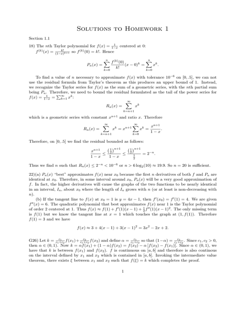
Solutions to Homework 1
Section 1.1
1
18) The nth Taylor polynomial for f (x) = 1−x
centered at 0:
k!
(k)
(k)
f (x) = (1−x)k+1 so f (0) = k!. Hence
Pn (x) =
n
X
f (k) (0)
k=0
k!
(x − 0)k =
n
X
xk .
k=0
To find a value of n necessary to approximate f (x) with tolerance 10−6 on [0, .5], we can not
use the residual formula from Taylor’s theorem as this produces an upper bound of 1. Instead,
we recognize the Taylor series for f (x) as the sum of a geometric series, with the nth partial sum
being Pn . Therefore,
P∞ kwe need to bound the residual formulated as the tail of the power series for
1
f (x) = 1−x = k=1 x :
∞
X
Rn (x) =
xk
k=n+1
which is a geometric series with constant
Rn (x) =
xn+1
∞
X
and ratio x. Therefore
xk = xn+1
k=n+1
∞
X
k=0
xk =
xn+1
.
1−x
Therefore, on [0, .5] we find the residual bounded as follows:
1 n+1
1 n+1
xn+1
2
2
≤
≤
= 2−n .
1
1−x
1−x
2
Thus we find n such that Rn (x) ≤ 2−n < 10−6 or n > 6 log2 (10) ≈ 19.9. So n = 20 is sufficient.
22)(a) Pn (x) “best” approximates f (x) near x0 because the first n derivatives of both f and Pn are
identical at x0 . Therefore, in some interval around x0 , Pn (x) will be a very good approximation of
f . In fact, the higher derivatives will cause the graphs of the two functions to be nearly identical
in an interval, In , about x0 where the length of In grows with n (or at least is non-decreasing with
n).
(b) If the tangent line to f (x) at x0 = 1 is y = 4x − 1, then f 0 (x0 ) = f 0 (1) = 4. We are given
f 00 (x) = 6. The quadratic polynomial that best approximates f (x) near 1 is the Taylor polynomial
of order 2 centered at 1. Thus f (x) ≈ f (1) + f 0 (1)(x − 1) + 21 f 00 (1)(x − 1)2 . The only missing term
is f (1) but we know the tangent line at x = 1 which touches the graph at (1, f (1)). Therefore
f (1) = 3 and we have
f (x) ≈ 3 + 4(x − 1) + 3(x − 1)2 = 3x2 − 2x + 2.
1
2
1
2
f (x1 )+ c1c+c
f (x2 ) and define α = c1c+c
so that (1−α) = c1c+c
. Since c1 , c2 > 0,
G26) Let k = c1c+c
2
2
2
2
then α ∈ (0, 1). Now k = αf (x1 ) + (1 − α)f (x2 ) = f (x2 ) − α [f (x2 ) − f (x1 )]. Since α ∈ (0, 1), we
have that k is between f (x1 ) and f (x2 ). f is continuous on [a, b] and therefore is also continous
on the interval defined by x1 and x2 which is contained in [a, b]. Invoking the intermediate value
theorem, there exists ξ between x1 and x2 such that f (ξ) = k which completes the proof.
1
Section 1.2
12) (a) With direct substitution we obtain the indeterminant form
0
0
so we employ L’hopital’s rule:
ex + e−x
ex − e−x
= lim
= 2.
x→0
x→0
x
1
lim
(b) f (.1) = 1.11−.905
= 2.05P
.100
(c) ex has Maclaurin series ∞
n=1
we obtain
1 n
n! x
so P3 (x) = 1 + x + 12 x2 + 61 x3 . With three digit rounding
P3 (.1) = 1.00 + .100 + .00500 + .000167 = 1.11
P3 (−.1) = 1.00 − .100 + .00500 − .000167 = .905
so f (.1) = 1.11−.905
= 2.05.
.100
(d) The relative error is
2.05−2.003335
2.003335
≈ .0233.
22) The nearest centimeter means the measurements fall into intervals:
3 ∈ [2.5, 3.5)
4 ∈ [3.5, 4.5)
5 ∈ [4.5, 5.5).
Hence the upper bound on the volume is the product of the largest possible values, 3.5 ∗ 4.5 ∗ 5.5 =
86.625 cm3 . Likewise the lower bound on volume is 2.5 ∗ 3.5 ∗ 4.5 = 39.375 cm3 . The upper and
lower bounds for the surface area are
2 (3.5 ∗ 4.5 + 3.5 ∗ 5.5 + 4.5 ∗ 5.5) = 119.5 cm2
and
2
2 (3.5 ∗ 4.5 + 3.5 ∗ 2.5 + 4.5 ∗ 2.5) = 71.5 cm .
Section 1.3
P
5
3
k x2k+1
6) The Maclaurin series for sin x is x − x3! + x5! − · · · = ∞
k=0 (−1) (2k+1)! . We use this in the
following parts.
1
1
1
1
(a) sin( n1 ) = n1 − 3!n
3 + 5!n5 − · · · so sin n = 0 + O( n ).
1
1
1
1
(b) sin( n12 ) = n12 − 3!n
6 + 5!n10 − · · · so sin n2 = 0 + O( n2 ).
2
(c) sin( n1 ) = 0 + O( n12 ) because
2 1
1
1
1
1
1
1
sin
=
−
+
− ··· ∗
−
+
− ···
n
n 3!n3 5!n5
n 3!n3 5!n5
1
2
=
−
+
·
·
·
.
n2 3!n4
(d) The Taylor series for ln x centered at 1 is
∞
ln x = (x − 1) −
X
(x − 1)2 (x − 1)3
(x − 1)k
+
− ··· =
(−1)k+1
.
2
3
k
k=1
1
Also ln(n + 1) − ln(n) = ln( n+1
n ) = ln(1 + n ). So for large n we have
1
1 1 1 2 1 1 3 1 1 4
ln(1 + ) ≈ −
+
−
+ ···
n
n 2 n
3 n
4 n
2
which clearly confirms limn→∞ [ln(n + 1) − ln(n)] = 0 and we have ln(n + 1) − ln(n) = 0 + O( n1 ).
P P
8) (a) For each i there are i multiplications in ni=1 ij=1 ai bj since j ranges from 1 to i. There are
P
exactly n iterations so there are a total of ni=1 i = n(n+1)
multiplications. There are i−1 additions
2
Pn
n(n−1)
for each i so there are a total of i=1 (i − 1) = 2 additions at each i. Then we must add these
sums together for n − 1 more additions. Therefore, there are n2 + n − 1 total computations.
(b) We can reduce the number of computations by writing this double sum in the form


n
i
X
X
ai
bj  .
i=1
j=1
Now there are still i − 1 additions for each i but only one multiplication. Then we must sum
+n+n−1 =
these terms resulting in n − 1 more additions. For this formulation there are n(n−1)
2
1
2 + 3n − 1) which is a reduction for n > 1.
(n
2
10) INPUT a, b, c (coefficients of a quadratic ax2 + bx + c)
OUTPUT x1 , x2 (roots of the quadratic)
If b = 0 q
q
−c
,
x
=
−
then x1 = −c
2
a
a .
else if b > 0
√
2
then x1 = − b+ b2a−4ac , x2 = − b+√b2c2 −4ac
else x1 = − b−√−2c
, x2 =
b2 −4ac
end
√
b− b2 −4ac
2a
end
OUTPUT(x1 , x2 ). STOP.
Note: There was some confusion on this problem. The text was asking about choosing the
best way to compute the output. If this was implemented in Matlab, for instance, you wouldn’t
need to tell it to compute an imaginary number as this would happen automatically. If you did this
in your psuedocode, that was fine. The key idea was when we should use the formulations based
on sgn(b).
Section 2.1
w −w
−g
−32.17 ew −e−w
e −e
20) We know 1.7 = x(1) = 2w
−
sin
w
.
Letting
f
(w)
=
−
sin
w
− 1.7
2
2
2
2
2w
we know that f (−1) = 3.67 > 0 and f (−.1) = −1.6 < 0. Therefore we utilize the bisection method
with intial interval [−1, −.1]. My algorithm provides the estimate p = −.317056 with error less
than or equal to .000003.
Section 2.2
8) g(x) = 2−x is continuous on [ 13 , 1]. g 0 (x) = −(ln 2)2−x and g is therefore decreasing on [ 13 , 1].
Since g(1) = .5 and g( 31 ) ≈ .7937, we have that for all x ∈ [ 31 , 1], .5 ≤ g(x) < .8 so that g :
[ 13 , 1] → [ 31 , 1]. Also, |g 0 (x)| = (ln 2) 2−x is also decreasing on [ 13 , 1]. Thus for all x ∈ [ 13 , 1],
1
|g 0 (x)| ≤ (ln 2) 2− 3 . Therefore, by Theorem 2.2, there is a unique fixed point in [ 13 , 1]. My algorithm
with tolerance 10−4 and initial approximation p0 = .5 returns p = .6412.
3
With my choice of p0 = .5 and k =
ln 2
1
, Cor. 2.4 provides
23
|pn − p| ≤
n 1
.
1
2
23
ln 2
n 1
So we want n such that ln12
2 < .0001. Using the properties of logarithms, we solve to see
23
that n > 14.253 is necessary. Therefore, we can expect an upper bound of 15 iterations.
Since the theoretical upperbound on the error is a worst case scenario, we anticipate that in
practice we will have smaller error. This should require us to need fewer iterations of the method.
In fact, my algorithm achieved the accuracy .0001 in 11 iterations.
20) Show that if A is any positive number, then the sequence defined by
1
A
xn = xn−1 +
, for n ≥ 1
2
2xn−1
converges to
√
A whenver x0 > 0.
√
Let g(x) = 12 x + A
A is a fixed point
x . Then xn = g(xn−1 ) defines the sequence and clearly
of g. We simply
√ want to show
√ that any initial, positive approximation will converge via fixed point
iteration to A. If x0 = A the sequence is constant and we are done.
h√
i
√
Suppose x0 ∈ ( A, ∞) and choose M > max {x0 , A, 1} so that x0 ∈
A, M . Note that
√
√
g 0 (x) = 21 1 − xA2 is defined on (0, ∞) and therefore on ( A, M ). For A < x < M , 0 < xA2 < 1
i
h√
A, M so that g is increasing.
and therefore |g 0 (x)| = 21 1 − xA2 < 12 (1) < 12 . Also g 0 (x) > 0 on
h√
i
h√
i
√
√
A
Since g( A) = A and g(M ) = 12 M + M
< 12 (M + 1) < M , then g :
A, M →
A, M .
h√
i
By Theorem 2.3 (Fixed-Point Theorem), for any intial approximation x0 ∈
A, M , the sequence
h√
i
√
xn = g(xn−1 ) converges to the unique fixed point A ∈
A, M .
√
√ 2
Now
that
√ suppose x0 ∈ (0, A). Since (x0 − A) > 0, we do the following calculation to show
√
x1 > A and therefore, the previous paragraph ensures convergence of xn = g(xn−1 ) to A.
√
√
x20 − 2x0 A
A
(x0 − A)2
0<
=
+
x0
x0
x0
√
A
= x0 +
−2 A
x0
√
√
= x1 − 2 A < x1 − A.
Thus x1 >
√
A.
G24) Let g ∈ C 1 [a, b] and p ∈ (a, b) be such that g(p) = p and |g 0 (p)| > 1. Show that there
exists a δ > 0 such that if 0 < |p0 − p| < δ then |po − p| < |p1 − p|. This implies that a fixed point
iteration following an approximation within δ of the root p will always be a worse approximation.
Thus, convergence won’t happen. We know that |g 0 (p)| = limp0 →p g(pp00)−g(p)
and so by definition, for any ∗ > 0 there exists a
−p
0 (p)| < ∗ .
δ ∗ > 0 such that |p0 − p| < δ ∗ implies that g(pp00)−g(p)
−
|g
−p
4
Let |g 0 (p)| = 1 + . From above, there is a δ > 0 such that if |p0 − p| < δ then
g(p0 ) − g(p) − (1 + ) < .
p0 − p Then
g(p0 ) − g(p) < 1 + 2
1<
p0 − p for all p0 ∈ [p−δ, p+δ]. Mulitplying the left inequality by |p0 −p| we have that for all p0 ∈ [p−δ, p+δ],
|p0 − p| < |g(p0 ) − g(p)| = |p1 − p| which establishes the claim.
5