Math 2250-4
Notes for Separable Differential Equations - %1.4
August 29, 2001
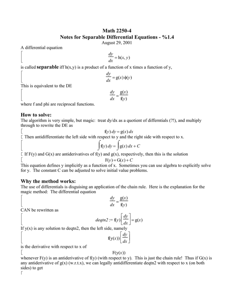
A differential equation
dy
= h(x, y )
dx
is called separable iff h(x,y) is a product of a function of x times a function of y,
dy
= g(x ) φ(y )
dx
This is equivalent to the DE
dy g(x )
=
dx f(y )
where f and phi are reciprocal functions.
How to solve:
The algorithm is very simple, but magic: treat dy/dx as a quotient of differntials (?!), and multiply
through to rewrite the DE as
f(y ) dy = g(x ) dx
Then antidifferentiate the left side with respect to y and the right side with respect to x.
⌠
⌠
f(y ) dy = g(x ) dx + C
⌡
⌡
If F(y) and G(x) are antiderivatives of f(y) and g(x), respectively, then this is the solution
F(y ) = G(x ) + C
This equation defines y implicitly as a function of x. Sometimes you can use algebra to explicitly solve
for y. The constant C can be adjusted to solve initial value problems.
Why the method works:
The use of differentials is disguising an application of the chain rule. Here is the explanation for the
magic method: The differential equation
dy g(x )
=
dx f(y )
CAN be rewritten as
 dy 
deqtn2 := f(y )   = g(x )
 dx 
If y(x) is any solution to deqtn2, then the left side, namely
 dy 
f(y(x ))  
 dx 
is the derivative with respect to x of
F(y(x ))
whenever F(y) is an antiderivative of f(y) (with respect to y). This is just the chain rule! Thus if G(x) is
any antiderivative of g(x) (w.r.t.x), we can legally antidifferentiate deqtn2 with respect to x (on both
sides) to get
F(y(x )) = G(x ) + C
which is what we got by magic before!
Example 1 page 31: We wish to solve
dy
= −6 x y
dx
y(0 ) = 7
Work:
Notice, our method for the general solution doesn’t actually give us the solution y(x)=0. Solutions
which exist to separable DE’s which are in addition to the ones we get are called "singular solutions."
slope field picture:
> restart:with(plots):with(DEtools):
Warning, the name changecoords has been redefined
> deqtn:=diff(y(x),x)=-6*x*y(x); #this is example 2
dsolve({deqtn,y(0)=7},y(x)); #Maple solution
DEplot(deqtn,y(x),x=-2..2,{[y(0)=7],[y(0)=-4]},y=-10..10,
arrows=line, color=black,linecolor=black,
dirgrid=[30,30],stepsize=.1,
title=‘Figure 1.4.1 page 31‘);
deqtn :=
∂
y(x ) = −6 x y(x )
∂x
y(x ) = 7 e
( −3 x 2 )
Figure 1.4.1 page 31
10
y(x)
–2
–1
5
0
1
x
2
–5
–10
Example extra:
dy
(2 / 3 )
=3y
dx
y(-1) = -1
Solution: (There is a twist to this problem that will let us discuss the existence-uniqueness theorem.)
> deqtn:=diff(y(x),x)=3*abs(y(x))^(2/3.0)*sign(y(x)):
DEplot(deqtn,y(x),x=-2..2,{[y(-1)=-1]},y=-5..5,
arrows=line, color=black,linecolor=black,
dirgrid=[30,30],stepsize=.1,
title=‘how many solutions really?‘);
how many solutions really?
4
y(x)
2
–2
–1
0
1
x
–2
–4
>
>
Example 3 page 32
> dy/dx=(4-2*x)/(3*y^2-5);
y(1)=3;
dy 4 − 2 x
=
dx 3 y 2 − 5
y(1 ) = 3
Work:
2
> restart:with(DEtools):with(plots):
Warning, the name changecoords has been redefined
> deqtn:=diff(y(x),x)=(4-2*x)/(3*y(x)^2-5):
DEplot(deqtn,y(x),x=-5..5,y=-5..5,
arrows=line, color=black,linecolor=black,
dirgrid=[40,40],stepsize=.1,
title=‘Figure 1.4.2 page 32 ‘);
>
Figure 1.4.2 page 32
4
y(x)
2
–4
–2
0
2
4
x
–2
–4
>