Modeling with first and second order systems of DE’s
Math 2250-4
Friday November 16, 2001
Example 1: Glucose-insulin model (adapted from a discussion on page 339 of the text "Linear
Algebra with Applications," by Otto Bretscher)
Let G(t) be the excess glucose concentration (mg of G per 100 ml of blood, say) in someone’s blood,
at time t hours. Excess means we are keeping track of the difference between current and equilibrium
("fasting") concentrations. Similarly, Let H(t) be the excess insulin concentration at time t. When blood
levels of glucose rise, say as food is digested, the pancreas reacts by secreting insulin in order to utilize
the glucose. Researchers have developed mathematical models for the glucose regulatory system. Here
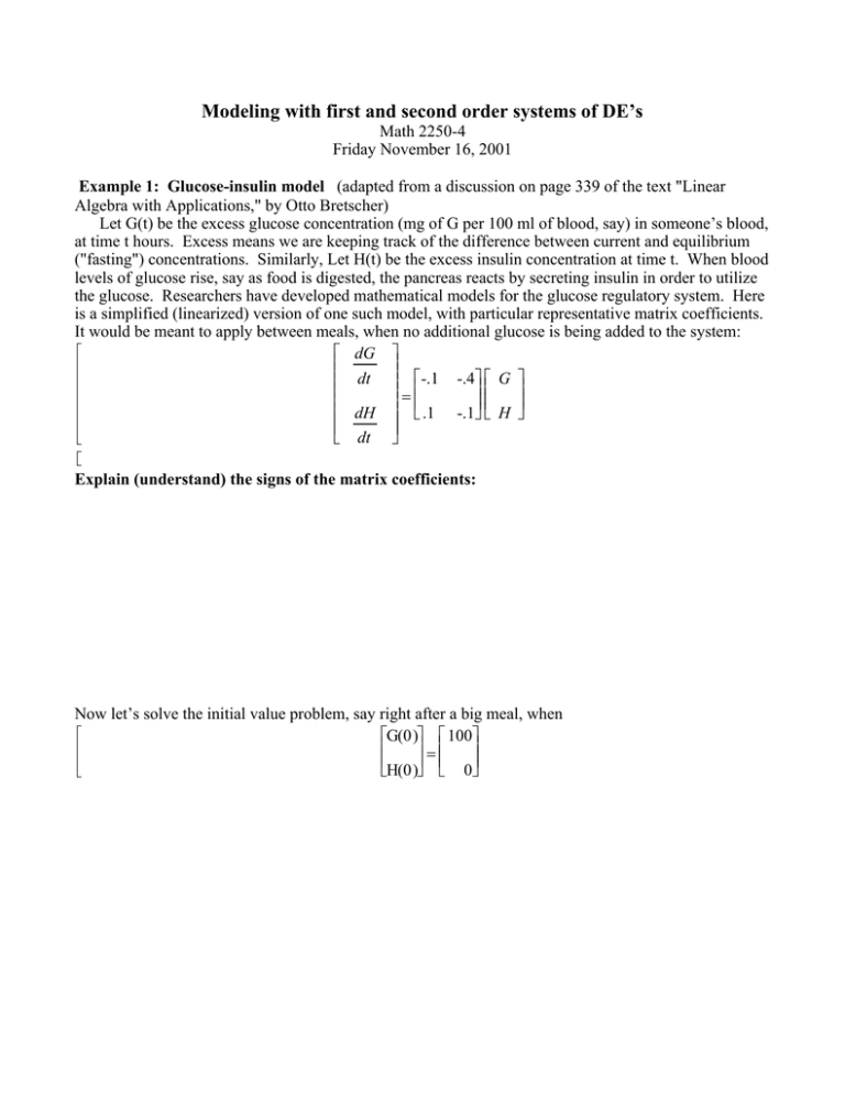
is a simplified (linearized) version of one such model, with particular representative matrix coefficients.
It would be meant to apply between meals, when no additional glucose is being added to the system:
 dG 


 dt   -.1 -.4  G 
 



=


 
 

 dH   .1 -.1  H 


 dt 
Explain (understand) the signs of the matrix coefficients:
Now let’s solve the initial value problem, say right after a big meal, when
G(0 )  100

 


 = 

H(0 )  0
> restart:with(linalg):with(plots):
> A:=matrix(2,2,[-.1,-.4,.1,-.1]);
 -.1 -.4

A := 

 .1 -.1
> eigenvects(A);
[-.1 + .2000000000 I, 1, {[-2.000000000 + 0. I, 0. + 1. I]}],
[-.1 − .2000000000 I, 1, {[-2.000000000 − 0. I, 0. − 1. I]}]
Extract a basis for the solution space to his homogeneous system of differential equations from the
eigenvector information above:
Solve the initial value problem.
Here are some pictures to help understand what the model is predicting:
(1) Plots of glucose vs. insulin, at time t hours later:
> G:=t->100*exp(-.1*t)*cos(.2*t):
H:=t->50*exp(-.1*t)*sin(.2*t):
> plot({G(t),H(t)},t=0..30,color=black,title=
‘Excess Glucose and Insulin concentrations‘);
Excess Glucose and Insulin concentrations
100
80
60
40
20
0
5
10
15
t
–20
20
25
30
2) A phase portrait of the glucose-insulin system:
> pict1:=fieldplot([-.1*G-.4*H,.1*G-.1*H],G=-40..100,H=-15..40):
soltn:=plot([G(t),H(t),t=0..30],color=black):
display({pict1,soltn},title=‘Glucose vs Insulin
phase portrait‘);
Glucose vs Insulin
phase portrait
40
30
H
20
10
–40
–20
20
40
60
G
–10
80
100
Example 2: Tanks: This is example 2 from our text, page 413. We have a cascade of three tanks, see
figure 7.3.2 page 413. The tank volumes are V1=20, V2=40, V3=50 (gallons). The water flow rate is
r=10 g/min. The initial amounts of salt are x1(0)=15, x2(0)=0, x3(0)=0.
Show that the initial value problem for this system is
 dx1 


 dt 
 -.5 0

0   x1 
 



 



 dx2  
 =  .5 -.25 0   x2 


 dt  


 



 

  0 .25 -.2  x3 

 dx3 


 dt 
x1(0 )  15

 


 




x2(0 ) =
  0


 


 

0
x3
(
0
)

 

Solve this system, using
> A:=matrix([[-.5, 0, 0], [.5, -.25, 0], [0, .25, -.2]]):
eigenvects(A);
[-.5, 1, {[1, -2.000000000, 1.666666667 ]}], [-.25, 1, {[0, 1, -5.000000000]}], [-.2, 1, {[0, 0, 1 ]}]
You should get
 3
 0
 0
x1(t )













( −.5 t ) 
( −.25 t ) 
( −.2 t ) 
 -6 + 30 e
 1 + 125 e
 0
x2(t ) = 5 e
























 5
 -5
 1
x3(t )
We can plot the three solute amount vs. time to see what is going on:
> x1:=t->15*exp(-.5*t):
x2:=t->-30*exp(-.5*t)+30*exp(-.25*t):
x3:=t->25*exp(-.5*t)-150*exp(-.25*t)+125*exp(-.2*t):
> plot({x1(t),x2(t),x3(t)},t=0..30,color=black,
title=‘salt contents in each tank‘);
salt contents in each tank
14
12
10
8
6
4
2
0
5
10
15
t
20
25
30
Example 3: Spring systems. This is Example 1 page 427. We have a mass-spring system with two
masses and two springs, see figure 7.4.3. m1=2, m2=1, k1=100, k2=50. Derive the second order
system Mx’’=Kx, i.e. equation (13) on page 427:
 d 2 x1 




2
 -150 50  x1 
0  dt
 2
 




 = 

 
 


2
1  d x2   50 -50  x2 
 0


2

 dt
which is equivalent to the system
 d 2 x1 




 dt 2  -75 25  x1 
 



 = 







 2
 d x2   50 -50  x2 


 dt 2 
This is like a single mass-spring equation, except now it’s a system.
What is the dimension of the solution space? (Hint: What size first order homogeneous system is it
equivalent to?).
If we look for solutions of the form cos(wt)*v, how is the angular velocity w related to eigenvalues of
the matrix A, where
> A:=matrix(2,2,[-75,25,50,-50]);
-75 25

A := 

 50 -50
> eigenvects(A);
[-25, 1, {[1, 2 ]}], [-100, 1, {[-1, 1 ]}]
Find the general solution, and explain geometrically, in terms of the springs, what’s going on: