STT 351 HW5
Due at the close of class 10 - 8 - 08.
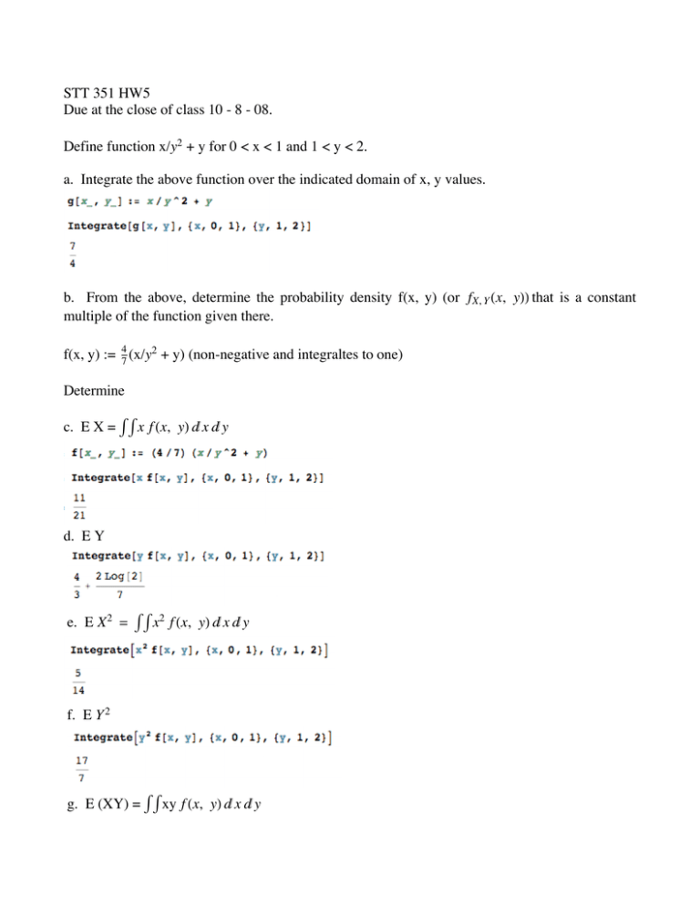
Define function x/y2 + y for 0 < x < 1 and 1 < y < 2.
a. Integrate the above function over the indicated domain of x, y values.
b. From the above, determine the probability density f(x, y) (or fX, Y Hx, yLL that is a constant
multiple of the function given there.
f(x, y) := 47 (x/y2 + y) (non-negative and integraltes to one)
Determine
c. E X = Ÿ Ÿ x f Hx, yL „ x „ y
d. E Y
e. E X 2 = Ÿ Ÿ x2 f Hx, yL „ x „ y
f. E Y 2
g. E (XY) = Ÿ Ÿ xy f Hx, yL „ x „ y
2
hw5key.nb
g. E (XY) = Ÿ Ÿ xy f Hx, yL „ x „ y
h. Var X
5/14 - H11 ê 21L 2
i. sX = sd X
root of (h)
j. Var Y
17/7 - H4 ê 3 + 2 HLog@2DL ê 7L 2
k. sY = sd Y
root of (j)
l. Covariance of X with Y defined by E(XY) - (E X)(E Y)
2
H7 + Log@4DL - (11/21) (4 ê 3 + 2 HLog@2DL ê 7L
21
m. Covariance of X with X
(7/4) - (11/21) (11/21) (just Var X)
n. Correlation between X, Y defined by
2
21
H7+Log@4DL-H11ê21L H4ê3 + 2 HLog@2DL ê 7L
5ê14-H11ê21L
2
17ê7-H4ê3 + 2 HLog@2DL ê 7L
E XY - HE XL HE Y L
sX sY
2
o. marginal density for X defined by fX HxL = Ÿ1 f Hx, yL „ y
2
for 0 < x < 1.
p. conditional density of y GIVEN x defined fy † xHyL =
f Hx, yL
fX HxL
for 0 < x < 1.
p. conditional density of y GIVEN x defined fy † xHyL =
f Hx, yL
fX HxL
hw5key.nb
3
q. conditional mean of y GIVEN x defined EIY † X = xL = Ÿ y fy † xHyL „ y
r. using the definitions, prove that in general E Y = E (E(Y † X)), i.e.
Ÿ y fY HyL „ y = Ÿ ( Ÿ y fy † xHyL „ y) fX HxL „ x
EY
E(Y † X = x)
Let's again calculate E Y directly from the joint density:
For comparison, calculate E Y from the marginal density for Y. In Mathematica it is neither
necessary nor convenient to use the subscripted notation fY HyLfor this density. We'll just have to
pay attention when using f[y] to denote this density in Mathematica.
Once again, we obtain the same expectation E Y by either of the two methods. But there is even
a third way to calculate E Y. It is to:
For each value X = x calculate the conditional expectation of Y for that value x. That
produces a function of x denoted E(Y † X = x). This fuction of x, when evaluated at random
variable X is denoted E(Y † X). The expectation of this r.v. is written E E(Y † X) and is
equal to E Y. This may seem puzzling because we are, in the final step, calculating E Y (a yintegral) as an x-integral
E Y = E E(Y † X) = Ÿ ‚ x fX HxL [ E(Y † X = x) ].
You can see why it works by carefully looking at the following. I'll use some additional brackets
[ E[Y † X = x ] ] to keep track of that portion of the integrand.
For each value X = x calculate the conditional expectation of Y for that value x. That
produces a function of x denoted E(Y † X = x). This fuction of x, when evaluated at random
variable X is denoted E(Y † X). The expectation of this r.v. is written E E(Y † X) and is
equal to E Y. This may seem puzzling because we are, in the final step, calculating E Y (a yintegral) as an x-integral
E Y = E E(Y † X) = Ÿ ‚ x fX HxL [ E(Y † X = x) ].
4
hw5key.nb
You can see why it works by carefully looking at the following. I'll use some additional brackets
[ E[Y † X = x ] ] to keep track of that portion of the integrand.
E[Y † X ] = Ÿ „ x fX HxL [ E(Y † X = x) ] = Ÿ „ x fX HxL [ Ÿ „ y y fY † X Hy † xL ]
= Ÿ „ x fX HxL [ Ÿ „ y y
fX, Y Hx, yL
fX, HxL
] = Ÿ „ x fX HxL [ Ÿ „ y y
fX, Y Hx, yL
fX, HxL
] =EY
Here is the calculation of E Y done htis third way:
E E(Y † X) above.
The whole idea of E Y = E E(Y † X) is really very simple. Say I want to calculate the mean of Y
= income next year taking into account X = income this year. I can calculate the mean of Y
specific to each possible value of X = x then weigh these according to the probabilities of these
different x.
Some motivational remarks.
Why study such a thing as E{Y † X) anyway?
Statistics is about expoiting simple relation ships of this kind. for example, there
is very general "Decomposition of Variance" formula we can easily prove once
we have the notios of conditional expectation and conditional variance in hand.
It is:
Var Y = E Var(Y † X) + Var( E(Y † X) )
I can briefly outline for you how this
"decomposition of variance Y in terms of X"
informs us how to design more efficient sampling methods.
Example: You have a budget of n = 100 samples from a population that is 34%
Hispanic. You can of course ignore that fact and just sample 100 people at random from your combined population of Hispanics and nonHispanics.
If you are interested in overall population mean income
know that the variance of your estimate is
Var
Y=
Var Y
100
=
sY 2
.
100
mY = E Y, you need to
Example: You have a budget of n = 100 samples from a population that is 34%
Hispanic. You can of course ignore that fact and just sample 100 peoplehw5key.nb
at ran-5
dom from your combined population of Hispanics and nonHispanics.
If you are interested in overall population mean income
know that the variance of your estimate is
Var
Y=
Var Y
100
=
mY = E Y, you need to
sY 2
.
100
Using the above "decomposition of variance" formula we can improve upon our
sampling effort.
If you can manage it, instead sample 34 (at random) from the subpopulation of
Hispanics and 66 from the subpopulation of non-Hispanics. If you do this, then
your overall sample mean Y * will have E Y * = overall population mean and Var
EIVarIY ¢ XL M
Y as a consequence of the forY* =
which is only one part of Var
100
100
mula above.
So it is best to divide the sample of 100, sampling 34 at random from Hispanics
and 66 at random from non-Hispanics, if possible, rather than to sample all 100
at random from the combined population!
The part of variance that dropped away when we chose to sample the "strata" of
VarI EIY ¢ XL M
Hispanics vs nonHispanics separately is
. So sampling strata
100
reduces variance to the extent that Hispanics have a different mean income than
the nonHispanics (i.e. E(Y † X = x) varies with X = 1 for Hispanics and X = 0 for
non-Hispanics).
These insights are possible precisely because we have the concepts of conditional
mean and conditional variance and the decomposition of variance which follows.