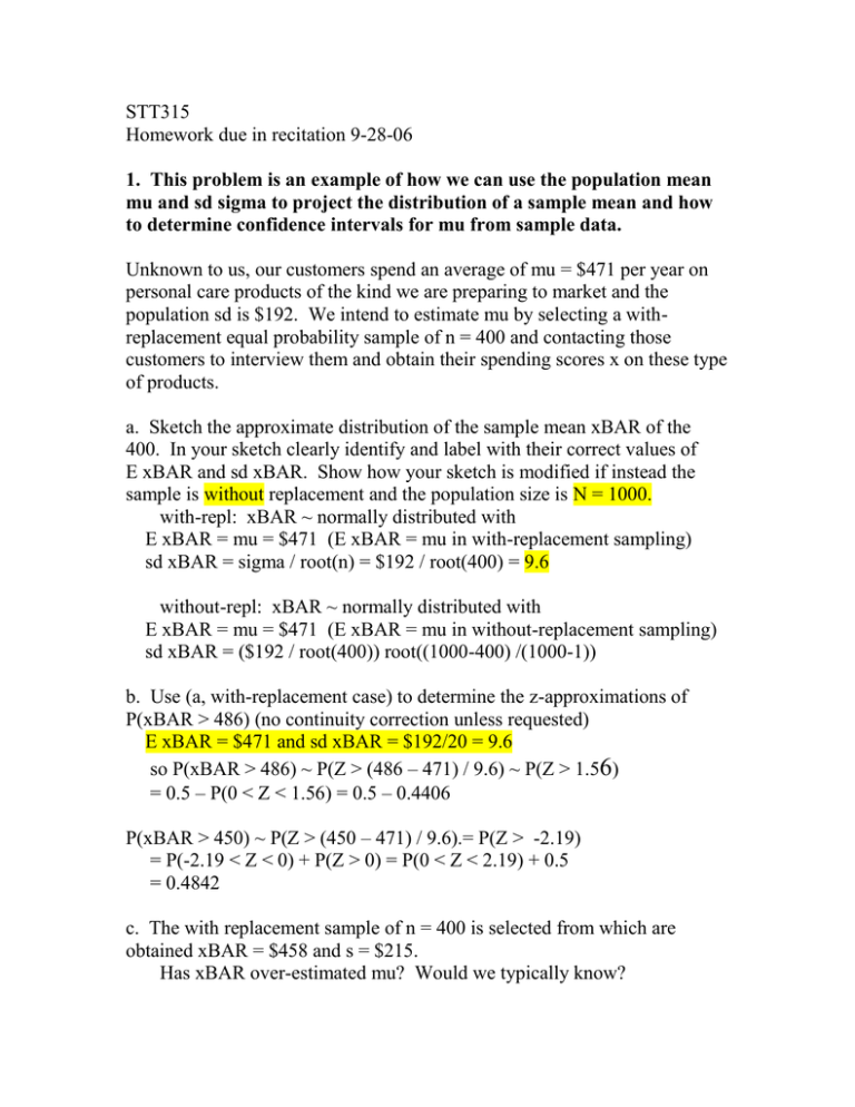
STT315
Homework due in recitation 9-28-06
1. This problem is an example of how we can use the population mean
mu and sd sigma to project the distribution of a sample mean and how
to determine confidence intervals for mu from sample data.
Unknown to us, our customers spend an average of mu = $471 per year on
personal care products of the kind we are preparing to market and the
population sd is $192. We intend to estimate mu by selecting a withreplacement equal probability sample of n = 400 and contacting those
customers to interview them and obtain their spending scores x on these type
of products.
a. Sketch the approximate distribution of the sample mean xBAR of the
400. In your sketch clearly identify and label with their correct values of
E xBAR and sd xBAR. Show how your sketch is modified if instead the
sample is without replacement and the population size is N = 1000.
with-repl: xBAR ~ normally distributed with
E xBAR = mu = $471 (E xBAR = mu in with-replacement sampling)
sd xBAR = sigma / root(n) = $192 / root(400) = 9.6
without-repl: xBAR ~ normally distributed with
E xBAR = mu = $471 (E xBAR = mu in without-replacement sampling)
sd xBAR = ($192 / root(400)) root((1000-400) /(1000-1))
b. Use (a, with-replacement case) to determine the z-approximations of
P(xBAR > 486) (no continuity correction unless requested)
E xBAR = $471 and sd xBAR = $192/20 = 9.6
so P(xBAR > 486) ~ P(Z > (486 – 471) / 9.6) ~ P(Z > 1.56)
= 0.5 – P(0 < Z < 1.56) = 0.5 – 0.4406
P(xBAR > 450) ~ P(Z > (450 – 471) / 9.6).= P(Z > -2.19)
= P(-2.19 < Z < 0) + P(Z > 0) = P(0 < Z < 2.19) + 0.5
= 0.4842
c. The with replacement sample of n = 400 is selected from which are
obtained xBAR = $458 and s = $215.
Has xBAR over-estimated mu? Would we typically know?
ans. No, 458 < 471 so xBAR has underestimated mu. We typically do not
know the population mean mu and so would not know that underestimation
has occurred.
Has s over-estimated sigma? Would we typically know?
ans. Yes, 215 > 192 so s has over-estimated sigma. We typically do not
know the standard deviation of the population scores and so wouuld have no
way of knowing the overestimation has occurred.
What is our estimate for the sd of xBAR?
ans. Theory tells us that the sd of xBAR is sigma / root(n) (in withreplacement sampling). If we have access to the sample of the population
we would estimate sigma ~ s = 215 (reported from the sample). Combining
these two fqacts we estimate the sd of xBAR to be ~ s / root(n) = 215 /
root(400) = 10.75.
d. Give the usual z-based 90% confidence interval for mu. Does it cover the
true mu? Would we typically know this?
ans. xBAR +/- z s / root(n) (i.e. est +/- z est of sd of est)
458 +/- 1.645 10.75
e. Give the usual z-based 90% confidence interval for mu if instead the
sample of 400 had been selected without replacement and the population
size is N = 1000.
ans. xBAR +/- z s / root(n) FPC (i.e. est +/- z est of sd of est)
458 +/- 1.645 10.75 root((1000-400) / (1000 – 1))
458 +/- 1.645 10.75 0.775
[444.295, 471.705]
f. What is the approximate value of P(mu in [ xBAR +/- 1.96 s / root(n) ])
for large n? ans. ~ 0.95
g. All else being equal, what happens to the width of a confidence interval if
the sample size is quadrupled?
ans. The width of the CI is reduced by a factor of two.
h. We desire a 95% confidence interval xBARFINAL n +/- 10 and are willing
to pay whatever it costs in terms of expanding our sample of 400 to some
possibly larger sample size “FINAL n.” What final sample size will do the
job? Consult section 6-6, but use s in place of sigma in formula (6-10) since
we typically do not know sigma but must estimate it as the value of our
sample sd s = $215 of the initial sample of 400.
ans. From formula (6-10)
FINAL n = (z s / B)2 = (1.96 215 / 10)2 ~ 1776.
If we do continue to sample up to this “FINAL n” sample size, and if we
should find that the sample mean out to this final sample size is $475, what
will be our 95% confidence interval for mu? Look at the first line of (h).
ans. We get the CI we desired (to within a rounding error caused by the fact
that the recommended final n from formula (6-10) may not be an integer).
xBAR (from final n) +/- 10
$475 +/- $10
[$465, $485]
We usually would not know if our CI was one of the 95% which are lucky
enough to cover the population mean mu. In this hypothetical problem
we’ve assumed at the outset that mu = $471. So our sample is in fact one of
the lucky 95% since 471 does belong to the CI [465, 485] produced by ur
sample.
2. This problem explores the use of a t-based confidence interval for the
mean mu of a normal population. As in (1) we will suppose that, not
known to us, the population mean mu is $471. Suppose now that the
population scores are (at least roughly) normal distributed and that a
sample of only n = 6 customers has produced a sample mean xBAR =
$458 and sample sd s = $215.
a. Use the t-table and the sample information just above to give a 90%
confidence interval for mu. Does this interval cover the true population
mean?
ans. Degrees of freedom = n – 1 = 6 – 1 = 5. t-table entry for df = 5 and
90% CI is found to be 2.015. Our 90% CI is
xBAR +/- t s / root(n)
458 +/- 2.015 215 / root(6)
[281.137, 634.863]
b. Refer to (b). Before the sample of n = 6 is selected what is the numerical
value of the probability P(mu in [ xBAR +/- 4.032 s / root(6) ])? ans. 0.90
3. This problem is an example of how we can use the population
proportion p to project the distribution of a sample proportion pHAT
and how to determine confidence intervals for p from sample data.
Unknown to us, 31% of our customers use a personal care product of the
kind we are preparing to market. We intend to estimate this p (which is p =
0.31 but we don’t know that) by selecting a with-replacement equal
probability sample of n = 400 and contacting those customers to interview
them and determine whether or not they use such a product.
a. Sketch the approximate distribution of the sample proportion pHAT for n
= 400. In your sketch clearly identify and label with their correct values of
E pHAT and sd pHAT. Show how your sketch is modified if instead the
sample is without replacement and the population size is N = 1000.
ans. with replacement:~ normal with
E pHAT = p = 0.31
sd pHAT = root(p q / n) = root(0.31 0.69 / 400) = 0.023
without replacement:~ normal with
E pHAT = p = 0.31
sd pHAT = root(p q / n) root((N-n) / (N-1))
= root(0.31 0.69 / 400) root(600 / 999)
= 0.023 0.775 = 0.018.
b. Without using any continuity corrections, use (a) in the with-replacement
case to determine the z-approximations of
P(pHAT > .28) ~ P(Z > (0.28 – p) / root(pq / n))
= P(Z > (0.28 – 0.31) / root(0.31 0.69 / 400))
= P(Z > -1.30) = 0.5 – P(0 < Z < 1.30)
= 0.5 – 0.4032 = 0.0968
P(pHAT < .34) ~ P(Z < (0.34 – 0.31) / root(.31 .69 / 400))
= P(Z < 1.30) = P(Z > -1.30) = 0.0968
c. A with replacement sample of 400 is selected, from which are obtained
130 customers who use a product of this type.
What is pHAT? Has it overestimated p? Would we typically know?
pHAT = 130 / 400 = 0.325 > p = 0.31, so yes, it has overestimated p
Typically we don’t know p and would be unaware that it had been
overestimated.
Using pHAT, what is our estimate of the population sd for score
x = 1 if use product of this type, x = 0 otherwise
ans. For x = 0 or x = 1 scores of which the fraction p score one the sd of the
population is root(pq) = root(0.31 0.69) in the case of this population.
What is our estimate for the sd of pHAT?
ans. The (theoretical) sd of pHAT is root(pq / n) (with repl case). Fopr this
population it is root(0.31 0.69 / 400) for with repl sample of n = 400.
d. Give the usual z-based 95% confidence interval for p. Does it cover the
true p? Would we typically know this?
ans. pHAT +/- 1.96 root(pHAT qHAT / n) for with repl sampling
= 0.325 +/- 1.96 root(0.325 0.675 / 400)
= 0.325 +/- 0.0459 (the “margin of error” is thus 0.459)
= [0.279099, 0.370901]
In around 95% of samples of 400 (with repl) the interval calculated in this
way from the sample will cover (enclose) the true value p = 0.31. If this
were a real sample we typically would not know p = 0.31 and would
therefore not be sure whether our CI was a “lucky one” containing p. As it
happens, in this made up example the CI did contain p = 0.31.
e. Give the usual z-based 95% confidence interval for p if instead the
sample of 400 had been selected without replacement and the population
size is N = 1000.
ans. pHAT +/- 1.96 root(pHAT qHAT / n) FPC for without repl sampling
= 0.325 +/- 1.96 root(0.325 0.675 / 400) root((1000-400) / (1000-1))
= 0.325 +/- 0.0356 (the “margin of error” is thus 0.0356, less than (d))
= [0.289428, 0.360572]
f. What is the approximate value of
P(mu in [ xBAR +/- 1.96 root(pHAT qHAT) / root(n) ]) for large n?
ans. 0.95 for with replacement sampling. Actually, the mathematical limit
is 0.95 as n tends to infinity (which it can because sampling is with
replacement).
g. All else being equal, what happens to the width of a confidence interval if
the sample size is quadrupled? ans. It is halved.
h. We desire a 95% confidence interval pHATFINAL n +/- 0.03 and are
willing to pay whatever it costs in terms of expanding our sample of 400 to
some possibly larger sample size “FINAL n.” What final sample size will
do the job? Consult section 6-6, but use pHAT qHAT (from our initial 400)
in place of pq in formula (6-11) since we typically do not know sigma but
must estimate it from the initial sample of 400.
ans. Formula (6-11) gives nFINAL = (1.96 root(pHAT qHAT) / 0.03)2
= (1.96 root(0.325 0.675) / 0.03)2 ~ 937
If we do continue to sample up to this “FINAL n” sample size of 937 (that
is, 537 in addition to the 400 w already have), and if we should find that the
pHAT from this final sample size is 0.321, what will be our 95% confidence
interval for mu? Look at the first line of (h).
ans. final pHAT +/- 0.03, just as we desired.
0.321 +/- 0.03
[0.291, 0.351]
By design, this is a relatively narrow (i.e. precise) CI and it can be said that
around 95% of those prepared in this way will cover p = 0.31. Ordinarily,
we do not know p and therefore do not know if p has been covered. Since
our example assumes p = 0.31 we observe that it has been covered by this
95% CI whose ME = 0.03 by design. But we had to pay the price of
continuing beyond our sample of 400 to a total of nFINAL = 937.
4. This problem is an example of how we can estimate the population
mean mu using a proportionally stratified sample and how to develop a
z-based confidence interval for this estimate. See the reading
assignment for this week.
Suppose that 40% of our customer population lives in a large city. We
decide to sample 400 customers in a stratified way by sampling 0.4 400 =
160 with repl from our customers living in a large city and the remaining
240 with repl from our customers who do not live in a large city. Our
findings from this sampling are
xBARcity = $453
xBARnoncity = $399
sCITY = $185
sNONCITY = $213
nCITY = 160
nNONCITY = 240
a. What is our estimate of mu1 = the mean yearly expenditures of large city
dwelling customers on products of the type we will be introducing?
ans. Our estimate of muCITY is xBARcity = $453.
b. What is our stratified estimate xBARSTRAT of mu = mean yearly
expenditures of our entire customer base on products of the type we will be
introducing?
ans. xBARstrat = 0.4 xBARcity + 0.6 xBARnoncity
= 0.4 453 + 0.6 399 = 420.6 dollars
Because we proportionally stratified our sample (by apportioning our perstratum sample sizes in proportion to their share of the population)
xBARstrat will just be the ordinary sample mean of the 400. BUT the 400
persons drawn into our stratified sample must give proportional
representation to city vs noncity, so sBARstrat cannot be analyzed as an
unrestricted with replacement or without replacement sample of 400.
c. Give the 95% z-based CI for mu using xBARSTRAT.
ans. xBARstrat +/-
1.96 root(W2 CITY s2 CITY / n CITY + W2 NONNITY s2 NONCITY / n
NONCITY)
420.6 +/1.96 root(.0.42 1852 / 160 + 0.62 2132 / 240)
420.6 +/- 19.822
[400.778, 440.422]
We have no way of knowing if this confidence interval (CI) contains the true
(overall) population mean mu. We can say that around 95% of all CIs
prepared in this way from proportionally stratified random samples will
cover the true mean.
NOTE: It is NOT technically correct so say that the given interval
[400.778, 440.422] contains mu with around 95% probability. After all, the
particular numerical interval is not random. The statement
P(mu in 95% CI) ~ 0.95
is correct since probability refers to the random sampling that produces the
random CI.
d. What advantage is claimed for using the above proportionally stratified
sampling approach to estimate mu instead of just taking a straight withreplacement n = 400 sample of the population and using muHAT?
ans. It tends to be narrower, for any overall sample size n, than the other CI
obtained by dispensing with stratification and just taking a with replacement
random sample of n from the entire population.
5. This problem is an example of how we can estimate the population
proportion p using a proportionally stratified sample and how to
develop a z-based confidence interval for this estimate. See the reading
assignment for this week.
Suppose that 40% of our customer population lives in a large city. We
decide to sample 400 customers in a stratified way by sampling 0.4 400 =
160 from our customers living in a large city and the remaining 240 from
our customers who do not live in a large city. Our findings from this
sampling are
39 of the 160 use a product of the type we will be introducing
92 of the 240 use a product of the type we will be introducing
a. What is our estimate of p1 = the proportion of large city dwelling
customers who use a product of the type we will be introducing?
p1HAT = 39 / 160 = 0.24375
b. What is our stratified estimate pHATSTRAT of p = proportion of our
entire customer base who use a product of the type we will be introducing?
pHATstrat = 0.4 39 / 160 + 0.6 92 / 240 = 0.3275
Owing to proportional stratification, this equals the overall proportion (39 +
92) / (160 + 240) of customers using a product of the given type (check it).
c. Give the 95% z-based CI for p using pHATSTRAT.
pHATstrat +/- 1.96
root(W2 CITY pHATCITY qHATCITY/ n CITY + W2 NONNITY
pHATNONCITY qHATNONCITY / n NONCITY).
0.3275 +/-
root(.42 (39/160 121/160) / 160 + .62 (92/240 48/240) / 240)
0.3275 +/- 0.0173
[0.3102, 0.3448]
d. What advantage is claimed for using the above proportionally stratified
sampling approach to estimating p, instead of just taking a straight n = 400
sample of the population and using pHAT?
ans. Generally narrower CI for the given sampling effort (but luck can
always come along to favor the poorer method).