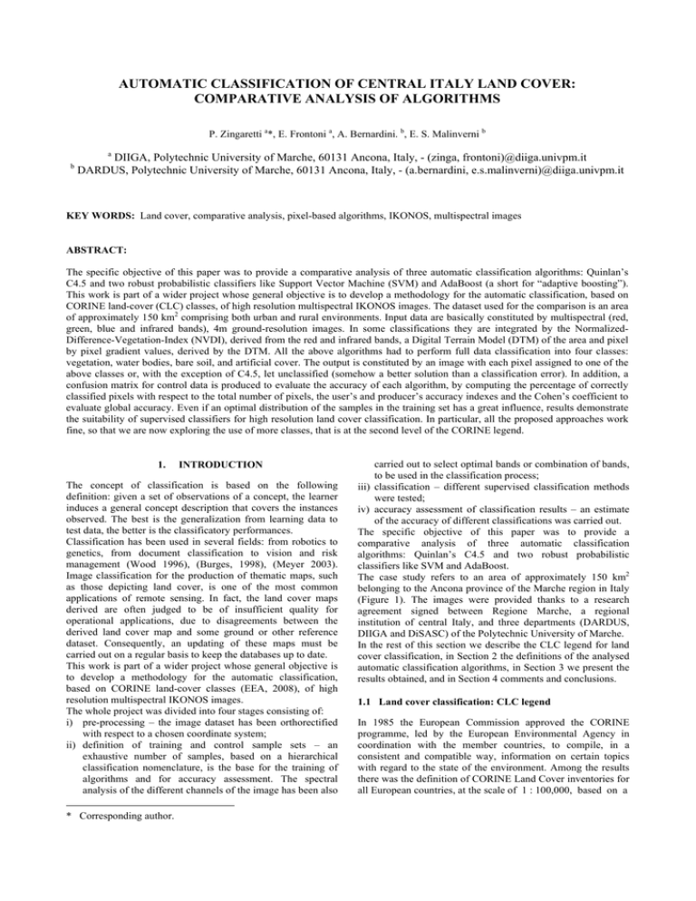
AUTOMATIC CLASSIFICATION OF CENTRAL ITALY LAND COVER:
COMPARATIVE ANALYSIS OF ALGORITHMS
P. Zingaretti a*, E. Frontoni a, A. Bernardini. b, E. S. Malinverni b
a
b
DIIGA, Polytechnic University of Marche, 60131 Ancona, Italy, - (zinga, frontoni)@diiga.univpm.it
DARDUS, Polytechnic University of Marche, 60131 Ancona, Italy, - (a.bernardini, e.s.malinverni)@diiga.univpm.it
KEY WORDS: Land cover, comparative analysis, pixel-based algorithms, IKONOS, multispectral images
ABSTRACT:
The specific objective of this paper was to provide a comparative analysis of three automatic classification algorithms: Quinlan’s
C4.5 and two robust probabilistic classifiers like Support Vector Machine (SVM) and AdaBoost (a short for “adaptive boosting”).
This work is part of a wider project whose general objective is to develop a methodology for the automatic classification, based on
CORINE land-cover (CLC) classes, of high resolution multispectral IKONOS images. The dataset used for the comparison is an area
of approximately 150 km2 comprising both urban and rural environments. Input data are basically constituted by multispectral (red,
green, blue and infrared bands), 4m ground-resolution images. In some classifications they are integrated by the NormalizedDifference-Vegetation-Index (NVDI), derived from the red and infrared bands, a Digital Terrain Model (DTM) of the area and pixel
by pixel gradient values, derived by the DTM. All the above algorithms had to perform full data classification into four classes:
vegetation, water bodies, bare soil, and artificial cover. The output is constituted by an image with each pixel assigned to one of the
above classes or, with the exception of C4.5, let unclassified (somehow a better solution than a classification error). In addition, a
confusion matrix for control data is produced to evaluate the accuracy of each algorithm, by computing the percentage of correctly
classified pixels with respect to the total number of pixels, the user’s and producer’s accuracy indexes and the Cohen’s coefficient to
evaluate global accuracy. Even if an optimal distribution of the samples in the training set has a great influence, results demonstrate
the suitability of supervised classifiers for high resolution land cover classification. In particular, all the proposed approaches work
fine, so that we are now exploring the use of more classes, that is at the second level of the CORINE legend.
1.
INTRODUCTION
The concept of classification is based on the following
definition: given a set of observations of a concept, the learner
induces a general concept description that covers the instances
observed. The best is the generalization from learning data to
test data, the better is the classificatory performances.
Classification has been used in several fields: from robotics to
genetics, from document classification to vision and risk
management (Wood 1996), (Burges, 1998), (Meyer 2003).
Image classification for the production of thematic maps, such
as those depicting land cover, is one of the most common
applications of remote sensing. In fact, the land cover maps
derived are often judged to be of insufficient quality for
operational applications, due to disagreements between the
derived land cover map and some ground or other reference
dataset. Consequently, an updating of these maps must be
carried out on a regular basis to keep the databases up to date.
This work is part of a wider project whose general objective is
to develop a methodology for the automatic classification,
based on CORINE land-cover classes (EEA, 2008), of high
resolution multispectral IKONOS images.
The whole project was divided into four stages consisting of:
i) pre-processing – the image dataset has been orthorectified
with respect to a chosen coordinate system;
ii) definition of training and control sample sets – an
exhaustive number of samples, based on a hierarchical
classification nomenclature, is the base for the training of
algorithms and for accuracy assessment. The spectral
analysis of the different channels of the image has been also
* Corresponding author.
carried out to select optimal bands or combination of bands,
to be used in the classification process;
iii) classification – different supervised classification methods
were tested;
iv) accuracy assessment of classification results – an estimate
of the accuracy of different classifications was carried out.
The specific objective of this paper was to provide a
comparative analysis of three automatic classification
algorithms: Quinlan’s C4.5 and two robust probabilistic
classifiers like SVM and AdaBoost.
The case study refers to an area of approximately 150 km2
belonging to the Ancona province of the Marche region in Italy
(Figure 1). The images were provided thanks to a research
agreement signed between Regione Marche, a regional
institution of central Italy, and three departments (DARDUS,
DIIGA and DiSASC) of the Polytechnic University of Marche.
In the rest of this section we describe the CLC legend for land
cover classification, in Section 2 the definitions of the analysed
automatic classification algorithms, in Section 3 we present the
results obtained, and in Section 4 comments and conclusions.
1.1 Land cover classification: CLC legend
In 1985 the European Commission approved the CORINE
programme, led by the European Environmental Agency in
coordination with the member countries, to compile, in a
consistent and compatible way, information on certain topics
with regard to the state of the environment. Among the results
there was the definition of CORINE Land Cover inventories for
all European countries, at the scale of 1 : 100,000, based on a
Figure 1. Case study: Italy, Marche region, Ancona province. On the right a panchromatic image of the area that has been processed.
standard methodology and nomenclature, for use with remote
sensing techniques. The CLC legend has a hierarchical structure
on three levels, containing 44 land cover classes grouped into
five major categories: 1. Urban Fabric, 2. Agriculture areas, 3.
Forest and semi-natural areas, 4. Wetlands, 5. Water bodies.
With respect of this structure, the high ground resolution of
current sensors, suitable for a map scale 1:10,000, suggested the
introduction of fourth and fifth level categories.
2. AUTOMATIC CLASSIFICATION ALGORITHMS
In this section, we describe the main classification methods that
will be used in this paper. We start by formally defining the
classification problem. Assume that we are given a training set
D, consisting of pairs <xi, li>, for i=1,2, … m. Each sample xi is
a vector in Rm that describes features joined to a certain
concept. The label li associated with xi is a binary or a multiple
label (for simplicity, we will discuss two-label classification
problems that can be easily generalized). A classification
algorithm is a function F that depends on two arguments, the
training set D and a query about xq that returns a predicted label
lq. We also allow for no classification to occur if xq is either
close to none of the classes or when it is too borderline for a
decision to be taken. Formally, this is realized by allowing the
label lq to be 0, 1 or 2, the latter representing an unclassified
query. Good classification procedures predict labels that
typically match the “true”, intended as ground truth, label of the
query. When unclassified is accepted as a possible output one
needs to consider the costs/penalties of the various outcomes in
analyzing the value of a classification method.
In our case <xi,li> are respectively a set of feature coming from
pixel based or region based analysis of multispectral images
joined, in some cases, with other pixel or region specific
characteristics (e.g. altitude, exposition, etc. ).
Here following we give a brief description of the three proposed
and tested classification methods: Quinlan’s C4.5, Support
Vector Machine (SVM) and AdaBoost.
2.1 - C4.5
The machine learning community has produced a large number
of programs to create decision trees for classification.
Noteworthy are Quinlan’s C4.5 (Quinlan, 1993), which is a
descendant of his earlier program ID3, and CART -
Classification And Regression Trees (Breiman, 1984), which is
a sophisticated program for fitting trees to data.
In general, tree-structured classifiers are constructed by making
repetitive splits of the measurement space X and the
subsequently created subsets of X, so that a hierarchical
structure is formed. It should be noted that when X is divided
into two subsets, these subsets do not both have to be
subsequently divided using the same variable, allowing
modelling a non homogeneous response. Besides, the
classification trees produced by tree-structured classification
methods are not guaranteed to be optimal: at each stage in the
tree growing process the split selected is the one that will
immediately increase the node purity the most (all cases from
the learning sample corresponding to the node belonging to the
same class); that is, on the contrary of using a tree-growing
program that “looks ahead”, which would require much more
time to create a tree, they are greedy algorithms.
C4.5 is a quite standard Decision Trees (Breiman, 1984) used as
general purpose learning technique for supervised
classification; it produces a flow chart like tree structure where
each node denotes a test on an attribute. Each branch represents
an outcome of the test and leaf nodes represent classes or class
distributions. In general the decision tree approach has several
disadvantages (multiple trees, variations) and the main
advantages are effectiveness and efficiency.
The basic algorithm to build decision trees uses a greedy
algorithm that constructs the tree starting from the top and then
goes down recursively by divide and conquer manner. C4.5
uses sophisticated pruning, and probabilistic facilities are used
to handle unknown and imprecise attribute values; unlike basic
approaches, C4.5 selects a working set of examples at random
from the training data and then tree growing/pruning process is
repeated several times to ensure that the most promising tree
has been selected.
2.2 - Support Vector Machine (SVM)
Support vector machines (SVMs) are a set of related supervised
learning methods used for classification and regression. They
belong to a family of generalized linear classifiers. They can
also be considered a special case of Tikhonov regularization. A
special property of SVMs is that they simultaneously minimize
the empirical classification error and maximize the geometric
margin; hence they are also known as maximum margin
classifiers.
Support vector machines map input vectors to a higher
dimensional space where a maximal separating hyperplane is
constructed. Two parallel hyperplanes are constructed on each
side of the hyperplane that separates the data. The separating
hyperplane is the hyperplane that maximizes the distance
between the two parallel hyperplanes. An assumption is made
that the larger the margin or distance between these parallel
hyperplanes the better the generalisation error of the classifier
will be. A tutorial has been produced by C.J.C Burges (Burges,
1998). A comparison of SVM to other classifiers has been made
by Meyer et al. (2003). An assessment of SVMs for land cover
classification is in Huang et al. (2002).
2.3 - AdaBoost
Boosting (Sutton, 2005) is a method of combining classifiers,
each of which iteratively created from weighted versions of the
learning sample, with the weights adaptively adjusted at each
step to give increased weight to the cases that were
misclassified on the previous step. The final predictions are
obtained by weighting the results of the iteratively produced
predictors. Boosting was originally developed for classification,
and is typically applied for creating an accurate strong classifier
by combining a set of weak classifiers. A weak classifier is only
required to be better than chance, and thus can be very simple
and computationally inexpensive. However, combining many of
them results in a strong classifier, which often outperforms most
“monolithic” strong classifiers such as SVMs and Neural
Networks. In 1990 Schapire (Schapire, 1990) developed the
predecessor to later boosting algorithms developed by him and
others. AdaBoost (a short for “adaptive boosting”) is now the
most popular boosting algorithm (Freund, 1997). Different
variants of boosting are known such as Discrete Adaboost, Real
AdaBoost, and Gentle AdaBoost (Schapire 1999). All of them
are identical with respect to computational complexity from a
classification perspective, but differ in their learning algorithm.
As already said, boosting uses a weighted average of results
obtained from applying a prediction method to various samples,
but the samples used at each step are not all drawn in the same
way from the same population, rather the incorrectly predicted
cases from a given step are given increased weight during the
next step. Thus boosting is an iterative procedure, incorporating
weights, as opposed to being based on a simple averaging of
predictions, as is the case with bagging (Sutton, 2005). In
addition, boosting is often applied to weak learners (e.g., a
simple classifier such as a two node decision tree), whereas this
is not the case with bagging.
AdaBoost is an algorithm for constructing a ”strong” classifier
as the linear combination
T
f ( x) = ∑ α t ht ( x)
t =1
of simple weak classifiers ht(x), which can be seen as basis
classifier, hypothesis or features. The strong classifier H derives
from the sign evaluation of the weak classifiers:
H ( x) = sign( f ( x))
The modified Real AdaBoost algorithm can be sketched as:
Modified Real AdaBoost algorithm
Input: Set of N labelled examples (x1, y1), . . . , (xN, yN), with
yi ∈ {−1, 1} , for 1 ≤ i ≤ N , xi ∈ ℜk , and where yi = +1 for
positive examples and yi = −1 for negative examples. xi is a
feature vector with k-components, each encoding a feature
relevant for the learning task.
Initialize weights D1(i) = 1/N
for t = 1, . . . , T do
1. Call the weak classifier ht(xi) that returns the minimum error
with respect to the distribution Dt;
It returns weak classifier ht : X ∈ {−1, 1} from H = {h(x)}
according to the following error function:
m
ht = arg min h ∈H ε j = ∑ i =1 Dt (i ) ⎡⎣ yi ≠ h j ( xi ) ⎤⎦
j
Dt (i ) ∗ e −α y h ( x )
zt
where zt is a normalization factor chosen so that Dt+1 is a
distribution.
2. Update Dt +1 (i) =
t i t
i
3. Choose the weight α t ∈ ℜ , so to greedily minimize Zt in
each step
end for
Output: The final strong classifier:
T
H ( x) = sign(∑ α t ht ( x))
t =1
It is important to notice that the complexity of the strong
classifier depends only from the weak classifiers.
The algorithm repeatedly selects a weak classifier hj(x) using a
distribution D over the training examples. The selected weak
classifier is expected to have a small classification error on the
training data. The idea of the algorithm is to modify the
distribution D by increasing the weights of the most difficult
training examples in each round. The final strong classifier H is
a weighted majority vote of the best T weak classifiers.
To deal with non binary results we used a chain of binary
classifier. A binary classifier Ci classifies data x into belonging
to either class Hi0 or class Hi1 (i.e. false or positive
classification). We assume each classifier Ck passes through
data that it classifies as belonging to class Hi0 only (this
approach is also named filtering classifier). In this way we
obtain a n-class classifier starting from a binary one.
3.
RESULT AND DISCUSSION
In this section, after a brief description of the dataset and of the
pre-processing operations, and the definition of the performance
measures, we report and comment the classification results for
the C4.5, SVM and Adaboost algorithms.
3.1 - Dataset, pre-processing and sample definition
The dataset used for the comparison is an area of approximately
150 km2, located near the Ancona city, comprising both urban
and rural environments, and with a topography that includes flat
areas, but also the Natural Park of the Conero mountain, with a
550 m elevation range.
IKONOS images were acquired in July 2006, with a 29 degrees
solar zenith angle. The dataset is composed by a panchromatic
image at a ground resolution of 1m and multi-spectral 4m
resolution data constituted by four bands: red, green, blue and
near-infrared. These data were integrated by a Digital Terrain
Model (DTM) of the area, derived from the Regional Technical
Map (CTR) at the scale 1:10,000, which, however, by
definition, does not consider artificial structures. In addition, in
some classifications we used pixel by pixel gradient values,
derived by the DTM, and the Normalized Difference
Vegetation Index (NVDI) derived from the red (r) and nearinfrared (nir) channels, according to the following formula:
NDVI =
nir − r
nir + r
During the pre-processing phase, first all the images were
orthorectified in the UTM N33 WGS84 System, using a rational
function model. Then a geometric correction was performed
using 15 control points and the third order degree polynomial
equations, giving an RMS error below 1 pixel (1 meter). A
radiometric interpolation by means of the nearest neighbour resampling method preserved the original image values. Finally,
the study area was extracted from a submap of the original
image.
A classification system should be informative, exhaustive and
separable (Jensen 1996, Landgrebe 2003). The first step to this
aim is the definition of a hierarchical classification structure,
principally based on the user’s needs and spatial resolution of
remotely sensed data. To fit a standard classification system we
planned to use the CLC legend, but adopting the extended
legend provided by the Italian agency for environmental
protection and technical services (Agenzia per la Protezione
dell'Ambiente e per i servizi Tecnici - APAT) for the
Agriculture areas and introducing new levels, based on the
spectral response of different materials, for Urban areas.
On the base of this structure, a sufficient and significant number
of training samples have to be defined. The software training
stage was carried out by means of about 100,000 sample points
grouped in 130 training sites. After a dedicated-GIS platform
implementation each sample was collected by means of specific
in field campaign and/or pan-sharpened IKONOS dataset visual
interpretation. The choice of the detail level of the samples (i.e.,
if belonging to the first or to the second level of the legend) was
carried out by class separability statistical measurements. This
also allowed to improve the training set by excluding sites with
spectral values largely ranging far from corresponding class
mean values.
3.2 - Performance measures
We decided to analyse all the three classification algorithms
while performing full data classification at the first level of our
land cover legend, that is, into four classes: vegetation (V),
artificial cover (A), water bodies (W) and bare soil (B). The
output is constituted by an image with each pixel assigned to
one of the above classes or, with the exception of C4.5, let
unclassified (somehow a better solution than a classification
error).
The quantitative evaluation of the accuracy of each algorithm
was made according to the values of the confusion matrixes
(Foody, 2002) resulting from control data classification. In
particular, each confusion matrix is constituted in our case by
the labels of the four classes plus the user’s accuracy index
(UA) as last column attribute and the label NC, corresponding
to not-classified pixels, plus the producer’s accuracy index (PA)
as further row attributes:
V
A
W
B
NC
PA
V
X11
X21
X31
X41
X51
PAV
A
X12
X22
X32
X42
X52
PAW
W
X13
X23
X33
X43
X53
PAB
B
X14
X24
X34
X44
X54
PAA
UA
UAV
UAW
UAB
UAA
Each Xi,j represents the number of pixels of a given class
(column label) classified as the row label, so that their sum
represents the total number (N) of control pixels. Consequently,
the percentages of correctly (CC) and erroneously (EC)
classified pixels are given, respectively, by:
EC = ∑ i =1 ∑ j =1, j ≠ i X
CC = ∑ i =1 X i ,i / N
4
4
5
i, j
/N
UA and PA are defined as the ratio between the total number of
pixels correctly assigned to a class with respect to the total
number of pixels assigned or, respectively, belonging to the
class:
UAi =
X i ,i
∑ j =1 X i, j
4
PAi =
X i ,i
∑
4
j =1
X j ,i
Finally, we used as a global accuracy index the Cohen’s K
coefficient (Rosenfield and Fitzpatrick-Lins, 1986), defined as:
N * ∑ i =1 X i ,i − S
4
K=
N −S
2
; S=
∑ (∑
4
4
i =1
j =1
X i , j * ∑ j =1 X j ,i
4
)
In short, while UA and PA make a survey on the behaviours of
different classes, K and percentage of correctly classified pixels
represent in a general way the performance of each algorithm.
3.3 - Quantitative comparison of algorithms
The output is constituted by an image with each pixel assigned
to one of the above classes or, with the exception of C4.5, let
unclassified (somehow a better solution than a classification
error). In our comparative analysis we took into great attention
UA and K. The first was used to evaluate which classes reveal
classification problems, the latter to give a comprehensive
evaluation of classification performance.
Algorithms were compared on three datasets: the first one (D1)
using only the four multi-spectral bands (“red”, “green”, “blue”
and “near IR”); while in the second dataset (D2) the NDVI
index for each pixel is added, and the last dataset (D3) uses the
previous five features plus the DTM and its gradient values.
The dataset and the algorithm used are appended to the name of
each classification test. For example, L0-D1-A means test L0
on dataset D1 using the Adaboost algorithm. For all tests the
number of control pixels is always N=24393.
In the following tables we report the confusion matrix values
for the most significant classification tests. Below each table the
performance measures defined in the previous section are
reported.
Table 1 and Table 2 report the results of two tests performed
using the Adaboost algorithm with the dataset D1 and D3,
respectively. Their comparison shows how, despite L0-D3-A
uses 7 features versus the 4 features of L0-D1-A, it gets lower
CC and K values. While this could be explained by the fact that
the DTM and its gradient values could be imprecise because
they do not consider artificial structures, it is more difficult to
explain why using the dataset D2 with the NDVI index in
addition to the 4 multi-spectral bands furnishes a similar result.
The same behaviour occurs also the C4.5 algorithm, while the
SVM algorithm generally gets, with respect to D1, greater K
but lower CC with D2, and very lower K and CC with D3.
Table 3 and Table 4 report the results of the two best
performing tests using C4.5 and SVM, respectively.
Figure 4 reports the classification results of the whole case
study area using the Adaboost algorithm, test L0-D1-A, while
in Figure 2 a zoomed part of it, near a small harbour, is shown.
the interpretation of the image is the following: V=green,
A=orange, W=blue, B=grey and NC pixels=white.
Figure 2. Portion of classification results for test L0-D1-A near
a small harbour: V=green, A=orange, W=blue and B=grey,
NC=white.
V
A
W
B
NC
PA
V
9362
0
2
3
10
99,84%
CC=95,39%;
A
4
1320
6
584
96
65,67%
W
3
2
11043
0
7
99,89%
EC=4,61%;
B
9
347
23
1543
29
79,09%
NC=0,58%;
UA
99,83%
79,09%
99,72%
72,44%
K=94,62%
Table 1. Confusion matrix and indexes for test L0-D1-A
V
A
W
B
NC
PA
V
9343
1
2
5
29
99,61%
CC=93,29%;
A
4
823
10
1060
113
40,95%
W
0
2
11045
0
8
99,91%
EC=6,71%;
B
22
238
12
1548
131
79,34%
NC=1,15%;
UA
99,72%
77,35%
99,78%
59,24%
K=89,43%
Table 2. Confusion matrix and indexes for test L0-D3-A
V
A
W
B
NC
PA
V
9333
0
2
42
0
99,53%
CC=95,30%;
A
37
1243
14
716
0
61,84%
W
0
3
11051
1
0
99,96%
EC=4,70%;
B
31
300
0
1620
0
83,03%
NC=0,00%;
UA
99,28%
80,40%
99,86%
68,10%
V
A
W
B
NC
PA
CC=95,67%;
A
5
1393
3
609
0
69,30%
W
0
5
11050
0
0
99,96%
EC=4,33%;
B
17
344
0
1590
0
81,50%
NC=0,00%;
4.
DISCUSSION AND CONCLUSIONS
The comparison of the results of three automatic classification
algorithms (C4.5, SVM and AdaBoost) over different datasets
has been presented. The comparison has been performed both
qualitatively (photo-interpretation by the superimposition of
classification results to an RGB or panchromatic image) and
quantitatively (using measures derived from the confusion
matrix).
Results demonstrate the suitability of supervised classifiers for
high resolution land cover classification. In particular, taking
the best performing tests of each algorithm the performances
are comparable (see Figure 3). However, the presence of not
classified data constitutes a good quality of the two
probabilistic approaches; usually in the classification literature
this kind of result is considered better than false and positive
results and usually not classified classes data are then
disambiguated using a second level classifier (different from the
first one) mixed with rule based approaches
In conclusion, even in presence of very small training sets the
proposed approaches work fine; so that we are now exploring
the use of more classes, that is at the second level of the
CORINE legend, and an optimal distribution of the samples in
the training set.
ACKNOWLEDGEMENTS
The authors would like to thank the Regione Marche for
providing the dataset used in the experiments.
K=93,79%
Table 3. Confusion matrix and indexes for test L0-D1-C
V
9304
0
36
37
0
99,22%
Figure 3. Cohen’s coefficient (K) and percentages of correctly
classified pixels (CC) in the test with best CC for each
algorithm (A=Adaboost, C=C4.5, S=SVM).
UA
99,76%
79,97%
99,65%
71,11%
K=94,25%
Table 4. Confusion matrix and indexes for test L1-D1-S
References
Breiman L., Friedman J.H., Olshen R.A., Stone C.J., 1984.
Classification and Regression Trees, Wadsworth, Pacific
Grove, CA.
Burges C.J.C., 1998. A Tutorial on Support Vector Machines
for Pattern Recognition, Data Mining and Knowledge
Discovery, 2, pp. 121–167.
European Environment Agency (EEA), CORINE Land Cover,
http://reports.eea.europa.eu/COR0-landcover/en (accessed 2
May 2008)
Figure 4. Classification results of the whole case-study area using the Adaboost algorithm: V=green, A=orange, W=blue, B=grey,
and NC= white.
Figure 5. Typical classification errors due to a great similarity between artificial cover and bare soil classes: the red pixels inside the
circle are erroneously classified as an artificial cover in image (a) on the left, and as bare soil in image (b) on the right.
Foody G.M., 2002. Status of land cover classification accuracy
assessment, Remote Sensing of Environment, 80, pp. 185–201.
Freund Y. and Schapire R.E., 1997. A decision-theoretic
generalization of on-line learning and an application to
boosting, Journal of Computer and System Sciences, 55(1), pp.
119–139.
Rosenfield, G. H. and Fitzpatrick-Lins, K. (1986). A coefficient
of agreement as a measure of thematic classification accuracy,
Photogrammetric Engineering and Remote Sensing, 52, pp.
223–227.
Schapire R., 1990. The strength of weak learnability, Machine
Learning, 5, pp. 197–227.
Huang C.; Davis L. S.; Townshend J. R. G., 2002. An
assessment of support vector machines for land cover
classification, Int. J. Remote Sensing, 23(4), pp. 725–749.
Schapire R.E. and Singer Y., 1999. Improved boosting
algorithms using confidence-rated predictions, Machine
Learning, 37(3), pp. 297–336.
Meyer D., Leisch F., and Hornik K., 2003. The support vector
machine under test, Neurocomputing, 55(1-2), pp. 169-186.
Sutton C.D., 2005. Handbook of Statistics, vol. 24, cap. 11:
Classification and regression trees, bagging, and boosting,
Elsevier, Amsterdam.
Quinlan J.R., 1993. C4.5: Programs for Machine Learning,
Morgan Kaufmann.
Wood J., 1996. Invariant pattern recognition: a review, Pattern
Recognition, 29(1), pp. 1-17.