Case Study in Data Analysis:
Does a drug prevent cardiomegaly in heart failure?
Harvey Motulsky
hmotulsky@graphpad.com
This is the first case in what I expect will be a series of case studies. It began when a GraphPad
customer (who wishes to be anonymous) asked for advice about how to analyze some data. I’d
appreciate suggestions for future case studies, and general ideas on how to make this kind of
case study more helpful. Please note that this kind of case study approach is necessarily
artificial, as I first analyze the data one way, and then another way, and then yet another way
Statistical analyses can only be interpreted at face value if all decisions about how to analyze
the data were made before the data were collected. The sequential approach used in this case
study is a reasonable way to analyze data from pilot experiments, but is not how actual data
should be analyzed.
In congestive heart failure, the heart muscle may get larger (myocardial hypertrophy) as a physiological
adaptation that allows the heart to pump enough blood to adequately perfuse the organs. With time, the
pumping chambers of the failing heart may weaken and dilate, resulting in not only a further increase in
heart size, cardiomegaly, but also a decreased ability to pump blood efficiently. Therefore, it makes sense
to seek a drug that would reduce cardiomegaly in heart failure.
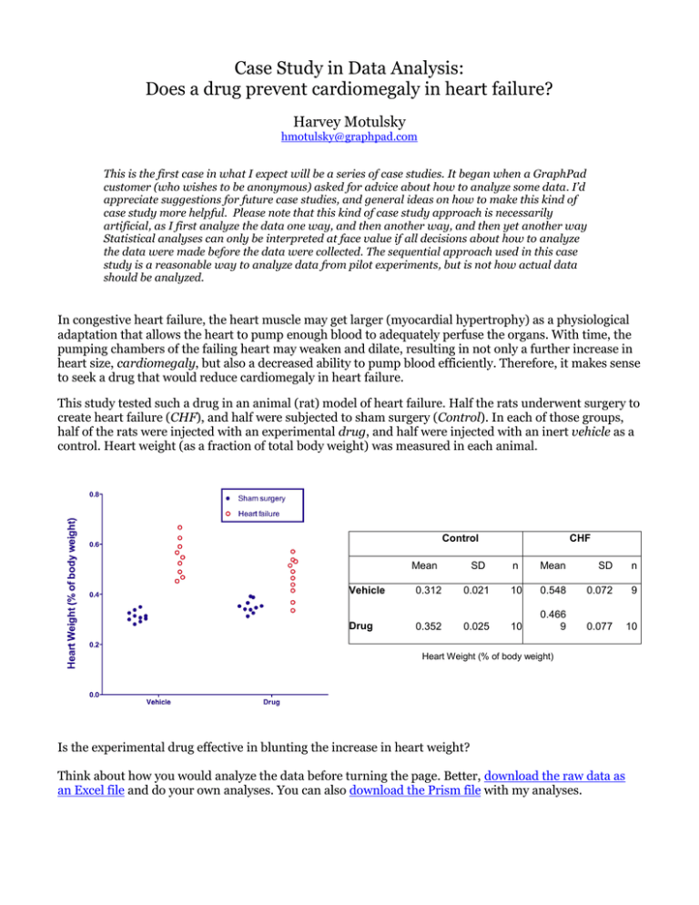
This study tested such a drug in an animal (rat) model of heart failure. Half the rats underwent surgery to
create heart failure (CHF), and half were subjected to sham surgery (Control). In each of those groups,
half of the rats were injected with an experimental drug, and half were injected with an inert vehicle as a
control. Heart weight (as a fraction of total body weight) was measured in each animal.
Control
Mean
CHF
SD
n
Mean
SD
n
Vehicle
0.312
0.021
10
0.548
0.072
9
Drug
0.352
0.025
10
0.466
9
0.077
10
Heart Weight (% of body weight)
Is the experimental drug effective in blunting the increase in heart weight?
Think about how you would analyze the data before turning the page. Better, download the raw data as
an Excel file and do your own analyses. You can also download the Prism file with my analyses.
FIRST IMPRESSIONS, BEFORE STATISTICAL ANALYSIS
Before doing analyses, it is always wise to carefully look at the data. Here are some thoughts:
 The heart-failure surgery does what it is supposed to do — induce heart failure, with a resulting
increase in heart weight. The mean heart weight of the vehicle-treated animals almost doubled
with the surgery. Since this is an established method, I’d want to compare these results with
results of prior runs of this experiment. Are these values similar to those commonly seen with this
kind of experiment? The investigators tell me that indeed these data match previous
experiments.
 The drug alone (i.e., in conjunction with sham surgery) increased heart weight, but this increase
is much smaller than that induced by the heart-failure surgery. This complicates the results. The
increase of heart weight with the heart-failure-inducing procedure is smaller in the drug-treated
animals. But this is partly because the drug increases heart weight in the sham-surgery group, and
partly because the drug decreases heart weight in the animals subjected to heart-failure surgery.
 The variation among values is much higher in the heart-failure-induced animals than in the
sham-operated animals. Presumably this is because of subtle differences in the surgery from one
animal to another, resulting in varying degrees of heart failure. This blurs the results a bit.
 There is a huge amount of overlap. Any conclusion will be about the differences between averages
of different experimental groups. The effect of the drug is not so pronounced that the heart weight
of every drug-treated animal is distinct from the heart weight of every control animal.
HOW TO DISPLAY DATA
The first step in using GraphPad Prism is to decide what kind of data table to use. This experiment is
defined by two grouping variables, so I entered the values into a Grouped data table in Prism. Half the
animals were subjected to surgery to create heart failure, and half underwent sham surgery. These two
groups define the two data-set columns. Half the animals were injected with an experimental drug, and
half were injected with vehicle as a control. These two groups define the two rows. Values from ten
animals (replicates) are placed side by side in subcolumns. One value was missing, and its spot is simply
left blank.
The preceding page displayed the raw data plotted from this grouped-data table. An alternative (and
more commonly used) approach is to create bar graphs (see below), plotting mean and SD (left), or mean
and SEM (right).
Copyright © 2010 GraphPad Software Inc. All rights reserved.
2
I prefer to see the actual data, as on page 1, when possible. With ten rats in each group, a graph of the raw
data is easy to understand, and is not excessively cluttered. I don’t see any advantage to plotting the mean
and SD or SEM, rather than the actual data.
It is also possible to plot both the raw data and the error bars on one graph, as shown below with SEM
error bars.
TWO-WAY ANOVA
The outcome (heart weight) is affected by two factors: whether or not the animal had surgically induced
heart failure, and whether or not the animal was given the drug. Therefore, my first thought was to
analyze the data by two-way ANOVA (later I’ll show alternatives).
Repeated measures ANOVA is not appropriate. Each animal underwent either surgery to create heart
failure or sham surgery, and received either the drug or the vehicle. No animal received two treatments
sequentially. This would be impossible, since the outcome being compared is the heart weight, which
cannot be determined while the animals are alive.
Copyright © 2010 GraphPad Software Inc. All rights reserved.
3
Here are the results of ordinary (not repeated measures) two-way ANOVA from GraphPad Prism:
Two-way ANOVA divides the total variation among values into four components:
Source of variation: Heart-failure-inducing surgery
The largest source of variation, determining 68.66% of the total variation, is the heart-failure-inducing
surgery.
This is not a surprise. The whole point of the experiment is to induce heart failure, which leads to larger
hearts. If an increase in heart weight did not result (in the control animals), we’d know something went
wrong with this particular experiment, and we wouldn’t even bother trying to make any conclusions
about the effect of the drug.
Two-way ANOVA reports a P value for this component of variation, but this P value is not helpful. It tests
the null hypothesis that, overall, the heart weights of the animals with surgically induced heart failure are
the same as the heart weights of the sham-operated animals. We know, for sure, that this null hypothesis
is false. There is no point in testing it, and its P value does not help answer the question this experiment
was designed to answer.
Source of variation: Drug
The second source of variation is the influence of the drug, accounting for only 0.98% of the total
variation. This analysis compares both groups treated with the drug (with or without heart failure) with
both groups not treated with the drug. This is not a particularly useful comparison. The P value tests the
null hypothesis that the drug has no effect on heart weight, averaging together the animals with surgically
induced heart failure and those without. I don’t see how this comparison is helpful, or how this P value
aids in interpreting the data.
Source of variation: Interaction
Interaction accounts for 8.12% of the total variability. The corresponding P value tests the null hypothesis
that there is no interaction; i.e., that the difference between the two surgery groups (heart failure versus
Copyright © 2010 GraphPad Software Inc. All rights reserved.
4
sham surgery) is the same regardless of the presence of drug. This would be equivalent to a null
hypothesis that the effect of the drug is the same in the two surgery groups. The P value is 0.0015. This is
easy to interpret. If this alternative null hypothesis of no interaction were true, there is a 0.15% chance
that random sampling would result in so much interaction (or more). Since this P value is tiny, we reject
the null hypothesis and conclude that the interaction is statistically significant.
We’ll continue the discussion of the interaction below.
Source of variation: Residual
The final source of variation is called residual or error. It quantifies the variation within each of the four
groups. There is no P value corresponding to the residual variation. Rather, the other three P values are
computed by comparing the three known sources of variation to residual variation.
Multiple comparison tests are not helpful
After ANOVA calculations, multiple comparisons tests often help you dig deeper to answer the relevant
scientific questions. Not here. As the data are entered, Prism can do two multiple comparison tests. It
can compute a confidence interval for the difference between the heart-failure and sham-surgery animals
that were treated with the experimental drug. And, it can do the same for the animals treated with the
vehicle.
If the data were transposed (which Prism can do using the Transpose analysis), the multiple comparison
tests could compute confidence intervals (and make decisions about statistical significance) for the
difference between experimental drug and vehicle for the animals with heart failure, and again for the
animals with sham surgery.
None of these four multiple comparison tests address the scientific question this experiment was
designed to answer. Multiple comparison tests are not helpful in this case, and are simply distractions.
Interaction confidence interval
Confidence intervals are much easier to understand than P values, but two-way ANOVA (in Prism, and in
most programs) doesn’t report a confidence interval for interaction. We can, however, calculate one.
The experimental question here is whether the difference in heart weights between heart-failure-surgery
animals and sham-operated animals given the drug is less than the difference in heart weights between
heart-failure-surgery and sham-operated animals given vehicle instead of drug.
Here are the mean heart weights (as percentage of body weight) in the four groups, the difference
between the animals with heart-failure surgery and sham surgery, and the difference of differences.
Heart-Failure Surgery
Sham Surgery
Difference
Diff. of differences
95% CI
Vehicle (no drug)
0.548
0.312
0.236
Experimental Drug
0.467
0.352
0.115
0.121
0.049 to 0.192
Since the confidence interval does not include zero, the P value must be less than 0.05. In fact, we have
already seen that the P value for interaction is 0.0015.
The Appendix explains how this confidence interval was computed.
Problems with using ANOVA to analyze these data
The discussion above finally arrived at an answer to the scientific question at hand. But, there are
problems with using ANOVA to analyze these data:
Copyright © 2010 GraphPad Software Inc. All rights reserved.
5
 The basic idea of ANOVA — partitioning the variation into components — is not a direct way to
answer the scientific question this experiment was designed to answer.
 Most of the ANOVA results are irrelevant to the scientific question.
 The terms effects and interactions are distracting. It is too easy thinking that the scientific goal of
this study (or others) is to seek effects or interactions, even when those values don’t correspond to
the scientific goals of the experiment.
 The confidence interval we need is not computed by two-way ANOVA (but, it isn’t hard to
compute by hand from the ANOVA results).
 Two-way ANOVA is based on the assumption that all the values are sampled from populations
that follow a Gaussian distribution, and that all four of these populations, whatever their means,
have the same SD. It takes only a glance at the raw data (page 1) to see that this assumption is
violated with these data. The scatter is much greater for the heart-failure animals with larger
hearts than it is for the animals given sham surgery.
ANALYZE THE DATA WITH REGRESSION
Entering the data on an XY data table
Since two-way ANOVA didn’t directly answer the experimental question, I switched to thinking about
models and regression. Below are the same data entered into an XY data table. The control (shamsurgery) animals are assigned an X value of 0; the heart-failure animals are assigned an X value of 1.
Copyright © 2010 GraphPad Software Inc. All rights reserved.
6
Analyze the data with linear regression
Here are the results of linear regression:
Since each line has only two X values, the best-fit lines go right through the mean value at each X. The Yintercepts are the Y values when X=0. Since X=0 is the code for sham-operated animals, the Y intercepts
equal the mean heart weight of sham-operated animals. The slope equals the difference between the
mean weight of the hearts of animals with heart-failure surgery and the mean weight of hearts of rats
given sham surgery, divided by the difference in X values. Since the two X values are 0 and 1, that
denominator equals 1. Each slope, therefore, equals the mean difference in heart weight, comparing
animals given heart-failure surgery to those given sham surgery.
The experimental question is whether the increase in heart weight was reduced in animals given the
experimental drug. This is equivalent to asking: Do the two slopes differ?
Prism doesn’t compute a confidence interval for that difference as part of linear regression analysis, but it
can compute a P value. Check the option in the Prism linear regression dialog to compare slopes and it
will report these results:
Are the slopes equal?
F = 11.867. DFn = 1 DFd = 35
P = 0.0015
Note that this F ratio and P value are identical to those reported by two-way ANOVA in testing the null
hypothesis of no interaction.
Here, linear regression really wasn’t a step forward. The value we care the most about — the difference
between the two slopes — was not computed by linear regression. Nor, was its confidence interval.
Many people find it hard to grasp the concept of interaction in two-way ANOVA. This example shows that
testing for interaction in two-way ANOVA (with two rows and two columns) is equivalent to testing
whether two slopes are identical. I think the idea of interaction is easier to understand in this context.
Analyze the data with “nonlinear” regression with equal weighting
Prism’s nonlinear regression analysis is far more versatile than its linear regression analysis. Let’s switch
to nonlinear regression, which can also fit straight lines.
Copyright © 2010 GraphPad Software Inc. All rights reserved.
7
Nonlinear regression lets you fit to user-defined models, so we can write a model that fits exactly what we
want to know — the difference between the two slopes. Here is the user-defined equation to be entered
into Prism’s nonlinear regression analysis:
<A>Slope = ControlSlope
<B>Slope = ControlSlope – DrugEffect
Y = Intercept + Slope*X
The last line is the familiar equation for a straight line. The two lines above it define the parameter Slope
for each data set. For the first data set (control animals given vehicle) we call the slope ControlSlope. For
the second data set, we define the slope to equal that control slope minus a parameter we call DrugEffect.
In the Constrain tab, define ControlSlope to be shared between the two data sets, so that Prism only fits
one value that applies to both data sets. This step is essential.
With this model, Prism fits the value we want to know, DrugEffect. It is the difference between the two
slopes, which is equivalent to the difference between the effect of heart failure in the controls (vehicle)
and the effect in the drug-treated animals.
Prism’s results:
The best fit value of DrugEffect is 0.121, with a 95% confidence interval ranging from 0.0495 to 0.192.
This is identical to the interaction confidence interval shown on page 5.
What about a P value? We can compare the fit of this model to the fit of a model where the DrugEffect is
forced to equal zero. Do this using the Compare tab of Prism’s nonlinear regression dialog:
Copyright © 2010 GraphPad Software Inc. All rights reserved.
8
The resulting P value is identical to what was obtained by ANOVA:
The F and P values are identical to the interaction results of two-way ANOVA results. But, there are three
advantages to using this model-fitting approach instead of ANOVA:
 It is easier to understand the results as a difference between two slopes than as an
interaction confidence interval.
 The confidence interval is computed as part of the nonlinear regression, so it doesn’t
require any manual calculations.
 As you’ll see below, the model-fitting approach (via nonlinear regression) gives us more
options.
Regression with differential weighting
ANOVA, as well as the regression analysis of the prior section, assumes that all four groups of data were
sampled from populations with identical standard deviations. This assumption is unlikely to be true.
Here are the sample standard deviations of the four groups:
Group
Sham surgery & Vehicle
Sham surgery & Drug
Heart failure & Vehicle
Heart failure & Drug
Mean
0.3124
0.3518
0.5481
0.4669
SD
0.02112
0.02508
0.07226
0.07677
%CV
6.76%
7.13%
13.18%
16.44%
Copyright © 2010 GraphPad Software Inc. All rights reserved.
9
The group of animals with heart failure has a larger standard deviation than the sham-surgery group.
This isn’t too surprising. The surgery to create heart failure is difficult, and tiny differences in the surgery
would result in different degrees of heart failure and different heart weights.
One way to cope with this situation is to apply weighting factors in the nonlinear regression. Standard
(unweighted) regression minimizes the sum of the squares of the difference between each observed value
and the value predicted by the model. The most common form of weighted regression effectively
minimizes the sum of the squares of the relative distance (the difference between the observed and
predicted value divided by the predicted value). This kind of weighting makes sense when the standard
deviations are not consistent, but the coefficients of variation (CV, which equals the SD divided by the
mean) are consistent.
With these data (see table above), the coefficients of variation are more consistent than the standard
deviations. But the CV is higher in the animals with heart failure than those without. The assumption
about consistent standard deviations (unweighted regression) or consistent coefficient of variation
(weighted regression) applies to the underlying populations. All we have here are the data from one
experiment. Ideally, we would want more data (from a number of experiments) before deciding how to
best weight the data. And, in addition to more data, it would be nice to have some theory about where the
variation is coming from.
For this analysis, I’ll assume that the CV is consistent (and that the variations we observed in CV values
are simply due to random sampling). Therefore, I chose Weight by 1/Y2 (minimize the relative distances
squared) on the Weights tab of Prism’s nonlinear regression dialog.
Copyright © 2010 GraphPad Software Inc. All rights reserved.
10
Since there are only two points on each line, the best fit lines don’t change with different weighting. But
using differential weighting does affect the P value and confidence interval. The P value testing the null
hypothesis that there is no drug effect equals 0.0008, giving us strong evidence to reject that null
hypothesis. The confidence interval for the drug effect ranges from 0.0553 to 0.186, a bit narrower than it
was with equal weighting.
Fitting a ratio rather than a difference
Expressing the effect of a drug as a difference in heart weight seems a bit awkward. Instead, let’s fit the
relative change in heart weight. The revised model is:
<A>Slope = ControlSlope
<B>Slope = ControlSlope * DrugEffectRatio
Y = Intercept + Slope*X
The last line is the familiar equation for a straight line. The two lines above it define the parameter Slope
for the two data sets. For the first data set (control animals given vehicle) we call the slope ControlSlope.
For the second data set, we define the slope to equal the control slope multiplied by a parameter we call
DrugEffectRatio.
In the Constrain tab, define ControlSlope to be shared between the two data sets. This instructs Prism to
use global fitting to only find one best-fit value for that parameter (not one for each line). This step is
essential.
With this model, Prism fits the value we really want to know, here called the DrugEffectRatio. It is the
ratio of the two slopes, which is equivalent to the ratio of the effect of heart failure in the control and
drug-treated animals.
Again, we’ll use relative weighting. The P value testing the null hypothesis that the DrugEffectRatio is
actually equal to 1.0 is 0.0008, the same as before. The best-fit value of the ratio is 0.488. In heartfailure-induced animals, the increase in heart weight in the drug-treated group equals 48.8 percent of the
increase in heart weight in the control (vehicle) group. The 95% confidence interval ranges from 0.278 to
0.698.
Expressed as a ratio, the results are easier to understand than when they were expressed as a difference.
In heart-failure animals, the presence of drug blunts the increase in heart weight to 48.8% of the increase
seen in control animals. The 95% confidence interval for that effect ranges from 27.8% to 69.8%. The P
value testing the null hypothesis that there is no drug effect is 0.0008.
A SIMPLER APPROACH: UNPAIRED t TEST
Problems with the ANOVA and regression approaches
Both the ANOVA and regression approaches analyze the data from all four groups of rats. Data were
collected from all four groups, so it seems reasonable to analyze all of the data. But, analyzing all of the
data leads to two unavoidable problems:
 The analyses are based upon an invalid assumption. ANOVA, and the simple approaches to
regression, assume that all four groups of data are sampled from populations with identical
standard deviations. A glance at the data (see graph on page 1) shows that this assumption is
violated. Weighted regression made an alternative assumption, but it is not at all clear that this
alternative assumption is valid.
 The drug has two effects. It decreases the heart weight in the animals with heart failure, but it also
increases the heart weights of the animals subjected to sham surgery. This complicates the
Copyright © 2010 GraphPad Software Inc. All rights reserved.
11
analysis, as both effects contribute to the outcome we are quantifying — the difference in heart
weight with heart failure, comparing animals treated with the experimental drug versus controls.
An alternative approach
At this point, I decided to use an alternative approach to reframe the experimental question, and simply
asked if the hearts of animals with heart failure are smaller when the animals are treated with the drug.
This analysis requires working with only two data sets:
An unpaired t test is based on the assumptions that both groups of data are sampled from populations
that follow a Gaussian distribution, and the SDs of both of these populations are identical (even if the
means are different). Both of these assumptions seem quite reasonable with these data. Therefore, the
two means can be compared with an unpaired t test.
The results are expressed both as a confidence interval, and as a P value:
 The difference between the two means is 0.0812, with a 95% confidence interval that extends
from 0.0088 to 0.154.
 The P value (two-tailed, testing the null hypothesis that the two populations have identical
means) equals 0.030. If the two populations really had the same mean, there is a 3.0% chance
that random sampling would result in a difference as large, or larger, than observed in this study.
The P value and confidence interval are consistent. Because the 95% confidence interval does not
include 0.0, the P value must be less than 0.05.
Expressing the results as a ratio
The results were expressed as a difference in weights (expressed as a percent of body weight), which is
not easy to think about. Dividing all the results by the mean weight of the control (vehicle) animals
converts the results into ratios that are easier to think about:
1. The difference between the mean heart weight of control and drug-treated is 0.0812.
2. Divide by the weight of the control animals, 0.548. The drug decreased the heart weight by
0.0812/0.548 = 14.8%.
Copyright © 2010 GraphPad Software Inc. All rights reserved.
12
3. The confidence interval of the difference ranges from 0.00883 to 0.154. Divide both of those
values by the weight of the control animals. The 95% confidence interval for the percent
reduction in heart rate ranges from 1.6% to 28.0%.
The mean heart weight of drug-treated animals was 14.8% smaller than the mean heart weight of the
control animals, with a 95% confidence interval ranging from 1.6% to 28.0%.
Statistical significance
The confidence interval and P value do a good job of summarizing the data. I don’t see that the concepts
of statistical significance are really useful with these data. But, most scientists prefer to label results as
statistically significant or not.
The P value is less than 0.05, so (using the conventional definition) these results can be deemed
statistically significant.
Scientific importance
Are these results scientifically important? Is the experiment worth repeating? The drug worked, and it is
unlikely to be a coincidence of random sampling. But the two groups of weights overlapped substantially.
The drug reduced the mean heart size by only 15%. Is that enough to be scientifically interesting?
The fact that the results are statistically significant really doesn’t help answer those questions. I can’t
answer them, because I don’t know enough about the physiology of heart failure, or about any other
drugs that ameliorate cardiomegaly. Those are scientific questions, not statistical ones. Don’t let the word
significant prevent clear scientific thinking.
P value: One- or two-tails?
The P value reported above, 0.03, is a two-tail P value. The interpretation is straightforward. If the null
hypothesis (the experimental drug had no impact on heart weight) were true, there is a 3.0% chance that
random sampling would results in a difference as large or larger than observed in this experiment. This
includes a 1.5% chance that random sampling would result in a difference as large as that observed here,
with the drug-treated animals having lower heart weights (as actually happened); and, also, a 1.5 %
chance that random sampling would result in a difference as large or larger than observed here, with the
drug-treated animals having larger heart weights (the opposite of what actually happened).
To use a one-tail P value, one must decide that before collecting data and after stating the direction of the
experimental hypothesis very clearly. This experiment was conducted with the expectation (or at least the
hope) that the drug would decrease heart weight in the animals with heart failure. One could justify a
one-tailed P value if you decided, before collecting data, that any change in the other direction (drugtreated animals have larger hearts) would be attributed to random sampling, declared to be not
statistically significant, and not pursued further. I suspect that if the data had shown a large effect in that
unexpected direction, the investigators would have been interested in pursuing the findings. For that
reason, I almost always prefer to use two-tail P values.
More about one- vs. two-tail P values.
Common misunderstandings about P values.
What about the two groups that are not included in the analysis?
While the t test analyzed only the two groups of animals with heart failure, the other two groups were not
totally ignored. Those groups serve as essential controls, analyzed informally. There would be no point in
comparing the two heart-failure groups without first determining that the heart weights are higher in the
heart-failure-induced animals, and that the experimental drug did not have a huge impact on the weight
of the sham-surgery animals (no heart failure).
Copyright © 2010 GraphPad Software Inc. All rights reserved.
13
SUMMARY
This case study meanders a bit. This is partly a choice I made, to include as many topics as possible. And
partly it reflects my own thinking. I started this case, thinking it was about two-way ANOVA. Then I
thought about the regression approaches. Only after working on this case for a while did I realize
analyzing two groups with a t test answers the scientific question without violating any assumptions.
Statistical analyses can only be interpreted at face value if the protocol for analyzing the data was fixed
before the data were collected. If you analyze the data first this way, then that way, it is far too easy to be
fooled — to get the results you want, regardless of what the data really show. I hope this case study
helped you review some principles of statistics. But, keep in mind that the approach to data analysis
demonstrated with this case – try this, then that, then something else – is appropriate only when
analyzing preliminary data.
More:
Download the raw data as an Excel file
Download the Prism file with graphs and analyses
Additional notes about this case-study.
Copyright © 2010 GraphPad Software Inc. All rights reserved.
14
APPENDIX. CALCULATING THE INTERACTION CONFIDENCE INTERVAL
Here again is the table from page 6.
Heart-Failure Surgery
Sham Surgery
Difference
Diff. of differences
95% CI
Vehicle (no drug)
0.548
0.312
0.236
Experimental Drug
0.467
0.352
0.115
0.121
0.049 to 0.192
The confidence interval is computed by the following steps:
1. Calculate the pooled SD. Two-way ANOVA doesn’t report this value — but it’s easy to compute.
The residual (or error) mean square reported on the ANOVA table is essentially a variance. The
residual mean square is 0.002985. Its square root equals 0.0546, which is the pooled SD.
The pooled SD in ANOVA
2. Compute the standard error of that difference, by dividing the pooled SD by the square root of the
sum of the reciprocals of sample sizes:
𝑆𝐸 =
𝑃𝑜𝑜𝑙𝑒𝑑 𝑆𝐷
1
1
1
1
+
+ +
𝑛𝑎 𝑛𝑏 𝑛𝑐 𝑛 𝑑
=
0.0546
1
1
1 1
10 + 10 + 10 + 9
= 0.035031
3. Calculate the number of degrees of freedom (df) as the total number of values (39 rats) minus the
number of groups (4). So df=35.
4. Find the critical value from the t distribution for 95% confidence and 35 df. This value can be
computed using the free GraphPad QuickCalc, using a table found in most statistics books
(including Appendix D of Intuitive Biostatistics, 2nd ed.), or by using this Excel formula:
=TINV(1.0 - 0.95, 35). The value is 2.0301.
5. Calculate the margin of error of the confidence interval. It equals the standard error (0.03503)
times the value from the t distribution (2.0301). The margin of error equals 0.0711.
6. Add and subtract the margin of error from the observed difference (0.121, see table at the top of
this page) to obtain the confidence interval, which ranges from 0.049 to 0.192.
Copyright © 2010 GraphPad Software Inc. All rights reserved.
15