SOFTWARE FOR CARTOGRAPHIC RASTER-TO-VECTOR CONVERSION
Laurence R. Moore
U.S. Geological Survey
1400 Independence Rd.
Rolla, Missouri 65401
ABSTRACT
Systems that capture digital cartographic data from maps usually require raster-to-vector
conversion. The speed of modern computers makes it possible to vectorize large data sets of
run-length encoded cartographic linework in a reasonable time. Thinned cartographic linework
can be vectorized in one pass through the raster data followed by one pass through the
resultant vectors. Software written in the C language provides a raster-to-vector conversion
that is fast and portable. Simple rule-based techniques in the design provide software
flexibility, which allows software tuning for particular applications.
Key Words: raster, vectorization, rule-based, sequential processing, C language
Parallel algorithms can be conceptually simple
but they can be inefficient on se'quential
'
processors. For small data sets this is not a
problem. But most useful cartographic data sets
are not small.
INTRODUCTION
Rotating-drum raster scanners provide an efficient
means of capturing digital cartographic data from
maps. Vector data formats allow digital
cartographic data to be structured and stored
efficiently. Converting digital data from raster
to vector format is therefore required in most
digital cartographic production systems.
~or.sequential
~s ~mportant.
operations the order of processing
Suppose that the points in a
digital image are to be processed row by row
beginning at the upper left. As soon as a
particular point is processed, its new value,
rather than the original value, is used in
processing any succeeding points.
This conversion has historically been a problem.
Because high-resolution cartographic data sets can
be extremely large, the conversion of raster data
to vector data requires large computers, long
processing times, or both.
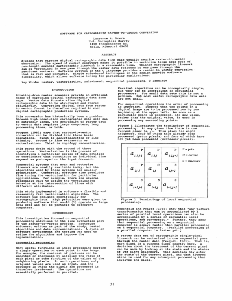
Figure 1 illustrates the terminology of sequential
processing. At any given time there is one
current pixel (a . . ). This pixel has eight
neighbors, four b~ which have already been
processed (prior pixels) and four of which have
not yet been processed (successor pixels).
Peuquet (1981) says that raster-to-vector
conversion can be divided into three basic
operations. First is skeletonization or line
thinning. Second is line extraction or
vectorization. Third is topology reconstruction.
This paper deals with the second of these
operations. Vectorization is the process of
identifying a particular series of data entities
or coordinates that constitute an individual line
segment as portrayed on the input document.
p
a 1' IJ'I
p
p
a· I ,
1- J
a 1-'1'1
J+
p .. prior
C ... current
S =- successor
Commercial systems that scan and vectorize
linework are readily available today, but the
algorithms used by these systems are usually
proprietary. Commercial software also precludes
fine tuning the vectorization for particular
applications. For example, there are several
reasonable ways to define the vectorization
behavior at the intersection of lines with
different attributes.
P
a
a l,}"1
S
a
This study implemented in software a flexible and
reasonably fast vectorization algorithm. The
software was designed specifically for
cartographic data. High priorities were given to
producing software that would (1) operate on large
data sets and (2) be portable to different
computers.
i+IJ-I
S
C
a"
1
lJ+
iJ
S
a
i+IJ
S
a
i+IJ+I
Figure 1 Terminology of local sequential
processing.
Rosenfeld and Pfaltz (1966) show that "any picture
by a
also be
accomplished by a series of sequential local
operations, ~nd conversely." Further, they show
that sequent~al processing on a sequential
computer is always faster than parallel processing
on a sequential computer.
(Parallel processing on
a parallel computer is faster yet.)
tra~sformation that can be accomplished
ser~es of parallel local operations can
METHODOLOGY
This investigation focused on sequential
processing solutions to the line extraction part
of the raster-to-vector problem. Prototype
softw~re, written as part of the study, tested
algor~thms and data representations.
A cycle of
software development and testing was used to
refine the algorithms and improve the
implementation.
A,raster data set of cartographic single-pixel
l~nework can be vectorized in one sequential pass
through the raster data (Peuquet, 1981). That is
eac~ ~ixel is a current pixel exactly once. A
'
dec~s~on about the treatment of the current pixel
can be made by looking at its state and the states
of its eight neighbors. This decision may alter
the state of the current pixel, and that altered
state is used for any subsequent processing that
involves the pixel.
Sequential processing
Manr useful functions in image processing perform
a s~ngle operation on each point in the image.
For example, the contrast of pictures can be
smoothed or sharpened by altering the value of
each pixel as some function of the values of the
ne~g~boring pixels.
In such operations, only
or~g~nal values are used as input, and. the
sequence in which the pixels are processed is
therefore irrelevant. The operations are
essentially performed in parallel.
31
Raster representation and processing
Each pixel in the current neighborhood has a color
(or attribute). This color either is the same as
the current pixel or is not the same as the
current pixel. These two possibilities can be
designated "1" and "0." The state of the
neighborhood can, therefore, be represented in a
single byte. Each bit shows the state of one of
the pixels in the eight-member neighborhood. This
one-byte coding of the neighborhood can be called
the neighborhood state. This is a meaningful
concept only if the current pixel is linework.
128
1
01000000
10000000
00000001
32
Figure 2
I
1
0
Do nothing
II
2
2
Make a node
III
3
1
Make a node
Close line of NE pixel
4
32
Make a node
Close line of W pixel
5
64
Make a node
Close line of NW pixel
6
128
7
5
8
34
Extend line of W pixel
9
66
Extend line of NW pixel
10
130
11
33
Connect line of W pixel
with line of NE pixel
12
65
Connect line of NW pixel
with line of NE pixel
13
160
Connect line of W pixel
with line of N pixel
14
37
Make a node
Close line of W pixel
Close line of NE pixel
15
69
Make a node
Close line of NW pixel
Close line of NE pixel
16
162
IV
Figure 2 shows the decimal and binary values of
each neighboring pixel. The neighborhood state is
calculated by summing the values of all linework
pixels. This coding scheme is taken from Greenlee
(1987), who credits the idea to Golay (1969).
Greenlee uses this neighborhood coding to reduce
storage space. The current study uses it to
reduce search times.
64
D
C
Raster cartographic linework is often stored using
run-length encoding to compress the data.
Run-length encoding is a good storage format, but
a poor processing format.
Sequential processing
software must use internal data representations
that simulate an uncompressed raster format.
V
VI
2
00100000
current
pixel
00000010
16
8
4
00010000
00001000
00000100
Table 1.
There are 256 possible neighborhood states (2 8 ).
This number is small enough to treat each one
individually.
In the worst case, no more than 256
rules are needed to define the vectorization of
all nine-pixel squares.
A rule set that dictates how specific
neighborhood states are handled.
3.
Information about the line membership
of the four predecessor pixels.
Rule numbers.
Column C: The one-byte decimal code of the
first (lowest-numbered) neighborhood state
to which the rule applies. Most rules apply
to more than one neighborhood state.
Table 2 relates all neighborhood codings to
the 16 rules.
Column D:
When the current pixel is not background, the
pixel must be assigned to a line. There are three
factors that affect this decision:
2.
Extend line of N pixel
Make a node
Close line of W pixel
Close line of N pixel
Rule set for sequent~al vector~zat~on.
Column B:
The raster data set is examined left to right and
top to bottom. Each pixel is the current pixel
only once. When the current pixel is part of the
map background, no action is taken and the scan
continues to the next pixel.
The neighborhood state.
Extend line of NE pixel
Column A: The 16 rules fall into six
categories. These categories are not
present in the software implementation of
the rules, but are useful to understanding
the system. For example, the four rules in
category IV can be generalized to "if there
is exactly one predecessor pixel, extend the
line containing that pixel to include the
current pixel."
Coding the neighborhood state.
1.
Make a node
Close line of N pixel
A brief statement of the rule.
The beginning and end of each line is flagged with
a node. The term node in this context does not
imply topologic structure. The raster processing
pass creates a node when two different vectors
meet or when a vector ends. Because the
processing is sequential, and because the
processor views only nine pixels at a time, large
numbers of temporary nodes are created.
For
example, a node will be created wherever there is
a local maximum or minimum in a line (Figure 3).
These temporary nodes must be removed during
subsequent processing. A node-line list and a
line-node list are constructed during the pass
through the raster data to aid vector processing.
These factors are applied in the order listed.
The first factor is the neighborhood state. This
is evaluated, and the result causes an appropriate
rule to fire.
The third factor to the vectorization decision for
the neighborhood is knowledge about the states of
other pixels in the neighborhood. The most
important piece of information is whether or not
any of these pixels are nodes. The words "close,"
"extend" and "connect" in table 1 mean different
things for nodes than for pixels.
The second factor is a vectorization rule set.
Sixteen rules are adequate for all 256
neighborhood states. Table 1 summarizes these
rules:
32
Rule
no.
1
0
2
234 678 10 11 12 14 15 16 18 19 20 22
23 24 26 27 28 30 31
3
1 21
4
32 42 43 46 47 48 56 58 59 60 62 63 96
106 107 110 111 112 120 122 123 124 126
127
5
64 74 75 78 79 82 83 84 86 87 88 90 91 92
94 95
6
128
148
195
214
7
5 9 13 17 25 29
8
34 35 36 38 39 40 44 50 51 52 54 55 98 99
100 102 103 104 108 114 115 116 118 119
9
66 67 68 70 71 72 76 80
10
vectors is a false node; the vectors that it
points to are combined and the traversal
continues. The traversal continues through nodes
recursively and ends when all lines that connect,
either directly or indirectly, to the start node
have been traversed.
Neighborhood states to which rule applies
129
149
199
215
131
150
202
218
135
151
203
219
138
154
206
222
Most cartographic data sets are not fully
connected graphs. The traversal of vectors is,
therefore, a series of graph traversals.
No linework coordinates have yet been removed from
the data set. The final step of the vector
processing is to remove coordinate values that are
not necessary to characterize the line. The
coordinates are filtered using the Douglas-Peucker
algorithm (Douglas and Peucker, 1973). The
resultant coordinates are sent to an output module
for storage.
139 142 143 146 147
155 158 159 192 193
207 210 211 212 213
223
RESULTS
The algorithms and structures described above were
implemented in software. The program is written
in ANSI C and is very portable.
It has been
tested on DOS (v3.3 and higher) PC's and on two
UNIX workstations.
Implementation
130 132 133 134 136 137 140 141 144 145
152 153 156 157 194 196 197 198 200 201
204 205 208 209 216 217 220 221
11
33 49 97 113
12
65
The three factors (neighborhood state, rule set,
predecessor pixels) to the vectorization process
are implemented as distinct processing steps.
First, the neighborhood state of the current pixel
is determined by an evaluation function.
13
160 161 176 177
14
37 41 45 53 57 61 101 105 109 117 121 125
15
69 73 77 81 85 89 93
Second, a function that codes one of the rules is
called. Each of the rules in table 1 is coded in
a C function. Although there are only 16 rules,
there are 256 possible neighborhood states. The
implementation uses an array of pointers to
functions to minimize the search time for the
appropriate rule.
I
162-175 178-191 224-255
16
Table 2. Ne~ghborhood states related to
vectorization rules.
Each element of an array of 256 pointers to
functions is initialized to point to the
appropriate rule (Figure 4). The result of the
evaluation of the neighborhood state becomes an
array index which permits the appropriate rule to
be called with a single array access.
Vector representation and processing
The sequential pass through the raster data set
associates each linework pixel with a vector line
string (except for cases where rule 1 is applied).
That is, the coordinates of the current pixel are
added to the coordinate list of some vector.
Third, a set of utility functions provides support
to the rule functions.
These utility functions
supply the intelligence of the third input to the
vectorization decision.
Production environment
The U.S. Geological Survey (USGS) uses its graphic
products as data sources for a variety of digital
products. Map separates are scanned at
resolutions of 750 or 1000 lines per inch. Such
data sets typically contain 250 to 450 million
pixels. Run-length encoding will usually compress
such data sets to less than 20 Mb. The goal of
this project was to produce nonproprietary
vectorization software that would operate directly
on these run-length encoded data sets.
connects to three
line strings
connects to one
line string
The software was designed to use relatively little
memory.
In general, directory structures (e.g.
node-line and line-node lists) are kept in memory,
but at anyone time the bulk of the coordinate
data are on the disk. The memory required by the
directory structures can be as high as 20 Mb for
large USGS maps scanned at high resolutions
(although less than 10 Mb is average), so it is
not practical to vectorize these very large data
sets on PC's. But UNIX workstations with 32 Mb or
more of memory can easily vectorize the largest
USGS data sets.
connects to two
line strings
Figure 3 Examples of node placement and line
string endpoint identification.
The output of the raster processing pass is a
vector data set that is not very useful.
It will
typically consist of a very large number of line
fragments that are tied together by temporary
nodes. Consolidating these fragments by removing
unnecessary nodes requires further processing of
the vector data.
Keeping coordinate data on disk instead of in
memory results in slower performance. But
vectorization is a batch process that takes a
small amount of time compared with the total time
and cost of producing a digital data set from a
map. On a 17-mip UNIX workstation, this software
will typically vectorize a 1:24,000-scale
quadrangle overlay in less than 1 hour.
The vector processing uses a form of a depth-first
search to visit all the coordinates ~n the data
set. Nodes that connect to exactly one vector, or
to more than two vectors, are true ends of lines.
These types of nodes are the starting points for
traversals of line strings. Any node found during
such a traversal that connects to exactly two
33
applicable to other aspects of cartographic raster
processing such as raster line skeletonization.
Test results
The largest data set tested with the software to
date is a topographic contour overlay of a USGS
1:100,000-scale quadrangle. This data set
contained more than 460 million pixels, of which
6.6 million were linework.
(The output vector
data set, stored in a relatively compressed binary
format, was about 1.7 Mb. The vectorization
process took about 85 minutes on a 17-mip
workstation. )
REFERENCES
Agrawala, Ashok K. and Ashok V. Kulkarni, 1977. A
sequential approach to the extraction of shape
features. computer Graphics and Image Processing,
6, pp. 538-577.
Douglas, David H. and Peucker, Thomas K., 1973.
Algorithms for the reduction of the number of
points required to represent a digitized line or
its caricature. The Canadian Cartographer, 10(2),
pp. 112-122.
In this test 111 of the 256 possible neighborhood
states were represented. However, only 11
neighborhood states accounted for 96 percent of
the actual neighborhoods, and 19 states accounted
for 99 percent of the actual neighborhoods.
Golay, M.J.E., 1969. Hexagonal parallel pattern
transformations. IEEE Transactions on computers,
C-18(8) •
1* prototypes of functions that comprise the
rules base *1
void rl(),r2(), 1* ... *1 r16();
Greenlee, David D., 1987. Raster and vector
processing for scanned linework. Photogrammetric
Engineering and Remote Sensing, 55(10), pp.
1383-1387.
1* array of 256 pointers to functions,
statically declared and initialized *1
void (*ruleFunc[256})() = {
Peuquet, Donna J., 1981. An examination of
techniques for reformatting digital cartographic
data/part 1: the raster-to-vector process.
Cartographica, 18(1), pp. 34-48.
rl, r3, r2, r2, r2, r7, r2, r2, r2, r7,
1* 240 more assignments go here *1
r16, r16, r16, r16, r16, r16
Rosenfeld, Azriel and Pfaltz, John L., 1966.
Sequential operations in digital picture
processing. Journal of the Association for
computing Machinery, 13(4), pp. 471-494.
};
1* program fragment to illustrate call to a
rule function *1
main ( )
(
int currState;
I * many lines of code here * I
1* evaluation of neighborhood state *1
currState = evaluate();
1* fire appropriate rule *1
(*ruleFunc[currState})();
1* many more lines of code here *1
}
Figure 4 Implementation of the rule set as an
array of pointers to functions.
Analysis of this and other test data sets suggests
the 16 rules identified in this paper define a
reasonable cartographic vectorization process.
However, the analysis also suggests that these
rules are not uniquely correct. Characteristics
of the output data can be changed relatively
easily by altering the rules. The speed and
efficiency can likely be improved by extending the
rule set to deal better with certain special
cases.
CONCLUSIONS
This research developed work of previous
investigators into a prototype software system.
cartographic vectorization requires only one
sequential pass through the raster data set.
Acceptable processing speeds do not require that
large amounts of the raster data be held in memory
at anyone time.
The nature of the vector output can be controlled
by a set of 16 rules. These rules can be coded in
software in a manner that makes them easy to
modify.
The 16 rules shown in table 1 work well on
cartographic data from USGS quadrangles. However,
these rules are probably not uniquely correct.
The behavior of the system can be modified by
changing these rules. It is probable that more
intelligence could be built into an extended rule
set to alter system behavior and improve
performance.
The combination of sequential processing and
rule-based decision making was quite effective in
this application. That combination may be
34