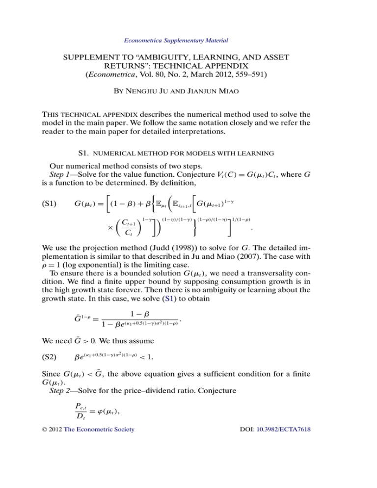
Econometrica Supplementary Material
SUPPLEMENT TO “AMBIGUITY, LEARNING, AND ASSET
RETURNS”: TECHNICAL APPENDIX
(Econometrica, Vol. 80, No. 2, March 2012, 559–591)
BY NENGJIU JU AND JIANJUN MIAO
THIS TECHNICAL APPENDIX describes the numerical method used to solve the
model in the main paper. We follow the same notation closely and we refer the
reader to the main paper for detailed interpretations.
S1. NUMERICAL METHOD FOR MODELS WITH LEARNING
Our numerical method consists of two steps.
Step 1—Solve for the value function. Conjecture Vt (C) = G(μt )Ct where G
is a function to be determined. By definition,
(S1)
G(μt ) = (1 − β) + β Eμt Ezt+1 t G(μt+1 )1−γ
Ct+1
×
Ct
1−γ (1−η)/(1−γ) (1−ρ)/(1−η) 1/(1−ρ)
We use the projection method (Judd (1998)) to solve for G The detailed implementation is similar to that described in Ju and Miao (2007). The case with
ρ = 1 (log exponential) is the limiting case.
To ensure there is a bounded solution G(μt ) we need a transversality condition. We find a finite upper bound by supposing consumption growth is in
the high growth state forever. Then there is no ambiguity or learning about the
growth state. In this case, we solve (S1) to obtain
Ḡ1−ρ =
1−β
1 − βe
(κ1 +05(1−γ)σ 2 )(1−ρ)
We need Ḡ > 0. We thus assume
(S2)
βe(κ1 +05(1−γ)σ
2 )(1−ρ)
< 1
Since G(μt ) < Ḡ the above equation gives a sufficient condition for a finite
G(μt )
Step 2—Solve for the price–dividend ratio. Conjecture
Pet
= ϕ(μt )
Dt
© 2012 The Econometric Society
DOI: 10.3982/ECTA7618
2
N. JU AND J. MIAO
where ϕ is a function to be determined. We substitute the return equation
Ret+1 =
Pet+1 + Dt+1 ϕ(μt+1 ) + 1 Dt+1
=
Pet
ϕ(μt )
Dt
into the Euler equation to derive
ρ−γ
−ρ Ct+1
Vt+1
1 = Et β
(S3)
Ct
Rt (Vt+1 )
1−γ −(η−γ)/(1−γ)
])
(Ezt+1 t [Vt+1
ϕ(μt+1 ) + 1 Dt+1
×
[Rt (Vt+1 )]−(η−γ)
ϕ(μt )
Dt
We use Vt = G(μt )Ct to derive
ρ−γ
1−γ −(η−γ)/(1−γ)
(Ezt+1 t [Vt+1
])
Vt+1
Rt (Vt+1 )
[Rt (Vt+1 )]−(η−γ)
⎞ρ−γ
⎛
Ct+1
)
G(μ
t+1
⎟
⎜
Ct
⎟
=⎜
⎝ Ct+1 ⎠
Rt G(μt+1 )
Ct
1−γ −(η−γ)/(1−γ)
Ct+1
Ezt+1 t G(μt+1 )
Ct
×
−(η−γ)
Ct+1
Rt G(μt+1 )
Ct
We substitute this equation into (S3) and then use the projection method to
solve for ϕ after we obtain the approximate solution for G in Step 1. We can
similarly solve for the price–consumption ratio.
S2. NUMERICAL METHOD FOR BENCHMARK MODEL I
In the paper, we also solve a benchmark model with Epstein–Zin preferences
under full information. We write the utility function as
1−ρ 1/(1−ρ)
Vt (C) = (1 − β)Ct1−ρ + β Rt (Vt+1 (C))
(S4)
1/(1−γ)
1−γ
(S5)
Rt (Vt+1 (C)) = Et [Vt+1
(C)]
Step 1. We conjecture the value function takes the form V (z) = G(z)Ct for
z = 1 2. The function G satisfies
1−γ (1−ρ)/(1−γ) 1/(1−ρ)
1−γ Ct+1
(S6)
G(z) = (1 − β) + β Ez G(z )
Ct
3
AMBIGUITY, LEARNING, AND ASSET RETURNS
That is,
(S7)
G(1)1−ρ = (1 − β) + β λ11 G(1)1−γ exp((1 − γ)κ1 + 05(1 − γ)2 σ 2 )
+ (1 − λ11 )G(2)1−γ
(1−ρ)/(1−γ)
× exp((1 − γ)κ2 + 05(1 − γ)2 σ 2 )
(S8)
G(2)1−ρ = (1 − β)
+ β (1 − λ22 )G(1)1−γ exp((1 − γ)κ1 + 05(1 − γ)2 σ 2 )
(1−ρ)/(1−γ)
+ λ22 G(2)1−γ exp((1 − γ)κ2 + 05(1 − γ)2 σ 2 )
We can solve this system of nonlinear equations for two unknowns G(1)
and G(2) We also need a transversality condition (S2).
Step 2. Given the solution for G(z) in Step 1, solve the price–dividend ratio.
Conjecture
Pet
= ϕ(zt )
Dt
where ϕ is a function to be determined. We substitute the return equation
Ret+1 =
Pet+1 + Dt+1 ϕ(zt+1 ) + 1 Dt+1
=
Pet
ϕ(zt )
Dt
into the Euler equation to derive
−ρ ρ−γ
Ct+1
Vt+1
ϕ(zt+1 ) + 1 Dt+1
1 = Et β
(S9)
Ct
Rt (Vt+1 )
ϕ(zt )
Dt
The above equation gives a system of two linear equations for two unknowns
ϕ(1) and ϕ(2). We check solutions such that ϕ(1) > 0 and ϕ(2) > 0
Dept. of Finance, Hong Kong University of Science and Technology, Clear Water Bay, Kowloon, Hong Kong and SAIF, Shanghai Jiaotong University, China;
nengjiu@ust.hk
and
Dept. of Economics, Boston University, 270 Bay State Road, Boston MA 02215,
U.S.A. and CEMA, Central University of Finance and Economics and AFR, Zhejiang University, China; miaoj@bu.edu.
Manuscript received December, 2007; final revision received June, 2011.