Avery I. McIntosh
Newton-Raphson for MAP estimates
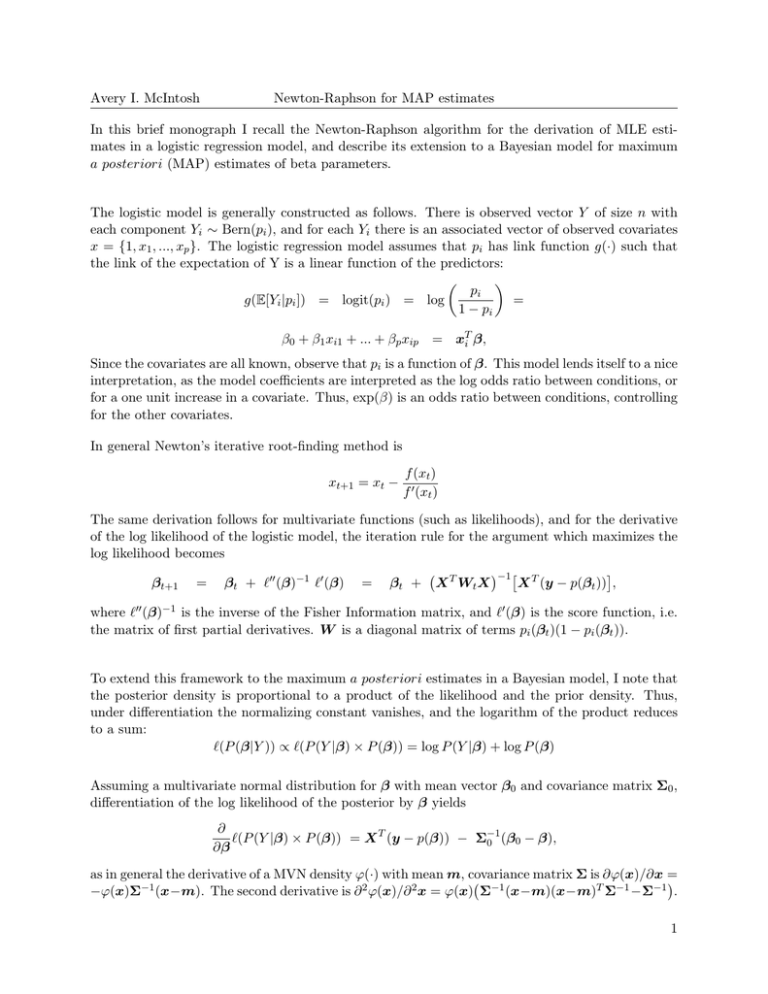
In this brief monograph I recall the Newton-Raphson algorithm for the derivation of MLE estimates in a logistic regression model, and describe its extension to a Bayesian model for maximum
a posteriori (MAP) estimates of beta parameters.
The logistic model is generally constructed as follows. There is observed vector Y of size n with
each component Yi ∼ Bern(pi ), and for each Yi there is an associated vector of observed covariates
x = {1, x1 , ..., xp }. The logistic regression model assumes that pi has link function g(·) such that
the link of the expectation of Y is a linear function of the predictors:
pi
g(E[Yi |pi ]) = logit(pi ) = log
=
1 − pi
β0 + β1 xi1 + ... + βp xip = xTi β,
Since the covariates are all known, observe that pi is a function of β. This model lends itself to a nice
interpretation, as the model coefficients are interpreted as the log odds ratio between conditions, or
for a one unit increase in a covariate. Thus, exp(β) is an odds ratio between conditions, controlling
for the other covariates.
In general Newton’s iterative root-finding method is
xt+1 = xt −
f (xt )
f 0 (xt )
The same derivation follows for multivariate functions (such as likelihoods), and for the derivative
of the log likelihood of the logistic model, the iteration rule for the argument which maximizes the
log likelihood becomes
−1 T
βt+1 = βt + `00 (β)−1 `0 (β) = βt + X T Wt X
X (y − p(βt )) ,
where `00 (β)−1 is the inverse of the Fisher Information matrix, and `0 (β) is the score function, i.e.
the matrix of first partial derivatives. W is a diagonal matrix of terms pi (βt )(1 − pi (βt )).
To extend this framework to the maximum a posteriori estimates in a Bayesian model, I note that
the posterior density is proportional to a product of the likelihood and the prior density. Thus,
under differentiation the normalizing constant vanishes, and the logarithm of the product reduces
to a sum:
`(P (β|Y )) ∝ `(P (Y |β) × P (β)) = log P (Y |β) + log P (β)
Assuming a multivariate normal distribution for β with mean vector β0 and covariance matrix Σ0 ,
differentiation of the log likelihood of the posterior by β yields
∂
`(P (Y |β) × P (β)) = X T (y − p(β)) − Σ−1
0 (β0 − β),
∂β
as in general the derivative of a MVN density ϕ(·) with mean m, covariance matrix Σ is ∂ϕ(x)/∂x =
−ϕ(x)Σ−1 (x−m). The second derivative is ∂ 2 ϕ(x)/∂ 2 x = ϕ(x) Σ−1 (x−m)(x−m)T Σ−1 −Σ−1 .
1
Avery I. McIntosh
Newton-Raphson for MAP estimates
Under the logarithm the second derivative of the MVN density is just −Σ−1 . Thus, the NewtonRaphson algorithm for the MAP estimators of a logistic model is modified in each component with
a term related to the prior:
−1 −1
T
−1
βt+1 = βt + X T Wt X + Σ
X
(y
−
p(β
))
−
Σ
(β
−
β)
t
|{z}
|
{z0
}
A sample R function for the method’s implementation follows. It takes as arguments a vector of
binary outcome values, a design matrix with intercept column, and a prior mean vector b0 and
prior covariance matrix S.
5
10
15
NRmap <- function(y,X,b0,S,start=1,tol=1e-6) {
B <- matrix(NA,ncol=1,nrow=ncol(X)) #matrix to store betas
B[,1] <- rep(start, ncol(X)) #starting values
i<-2
repeat {
p <- plogis(X %*% B[,i-1])
W <- diag(c(p*(1-p)))
S.inv <-solve(S)
score <- crossprod(X,(y - p)) - S.inv%*%(as.matrix(B[,i-1]-b0))
increm <- solve(crossprod(X,W)%*%X + S.inv)
B <- cbind(B,B[,i-1]+increm%*%score)
if (all(abs(B[,i]-B[,i-1]) < tol)) break
if (i>300) stop("Failure to find root after 300 iterations.
Attempt different starting value.")
i<-i+1
}
list(beta=t(B)[nrow(t(B)),], iterations=i-1)
}
2