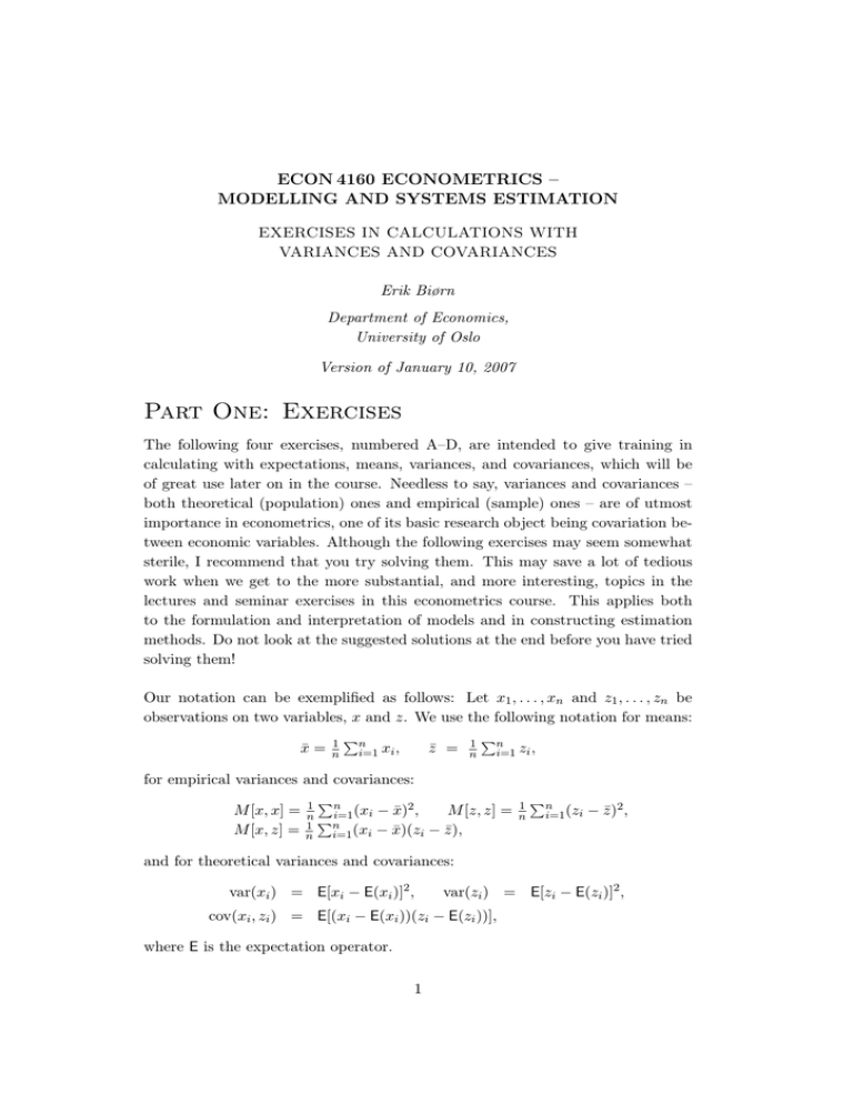
ECON 4160 ECONOMETRICS –
MODELLING AND SYSTEMS ESTIMATION
EXERCISES IN CALCULATIONS WITH
VARIANCES AND COVARIANCES
Erik Biørn
Department of Economics,
University of Oslo
Version of January 10, 2007
Part One: Exercises
The following four exercises, numbered A–D, are intended to give training in
calculating with expectations, means, variances, and covariances, which will be
of great use later on in the course. Needless to say, variances and covariances –
both theoretical (population) ones and empirical (sample) ones – are of utmost
importance in econometrics, one of its basic research object being covariation between economic variables. Although the following exercises may seem somewhat
sterile, I recommend that you try solving them. This may save a lot of tedious
work when we get to the more substantial, and more interesting, topics in the
lectures and seminar exercises in this econometrics course. This applies both
to the formulation and interpretation of models and in constructing estimation
methods. Do not look at the suggested solutions at the end before you have tried
solving them!
Our notation can be exemplified as follows: Let x1 , . . . , xn and z1 , . . . , zn be
observations on two variables, x and z. We use the following notation for means:
x̄ =
1
n
Pn
i=1 xi ,
z̄ =
1
n
Pn
i=1 zi ,
for empirical variances and covariances:
M [x, x] =
M [x, z] =
1 Pn
2
n P i=1 (xi − x̄) ,
n
1
i=1 (xi − x̄)(zi
n
M [z, z] =
− z̄),
1
n
Pn
i=1 (zi
− z̄)2 ,
and for theoretical variances and covariances:
var(xi ) = E[xi − E(xi )]2 ,
var(zi ) = E[zi − E(zi )]2 ,
cov(xi , zi ) = E[(xi − E(xi ))(zi − E(zi ))],
where E is the expectation operator.
1
Exercise A
Given the equations
(1)
(2)
yi = α + β xi + γ zi ,
wi = δ + ε xi + η zi ,
i = 1, . . . , n,
i = 1, . . . , n,
where yi , wi , xi and zi are considered as stochastic variables and α, β, γ, δ,
ε and η as constants. Prove, by using the definitions of theoretical variances
and covariances, that (1) imply the following relationships between theoretical
variances and covariances:
(a)
(b)
(c)
var(yi ) = β 2 var(xi ) + 2βγ cov(xi , zi ) + γ 2 var(zi ),
cov(yi , xi ) = β var(xi ) + γ cov(zi , xi ),
cov(yi , zi ) = β cov(xi , zi ) + γ var(zi ).
Further, show, by using (1) and (2), that the theoretical covariance between yi
and wi can be expressed in terms of var(xi ), var(zi ) and cov(xi , zi ) as follows:
(d) cov(yi , wi ) = β ε var(xi ) + (β η + γ ε) cov(xi , zi ) + γ η var(zi ).
Note that (d) is a generalization of (a).
Exercise B
Similar relationships as in exercise A also hold for empirical variances and covariances. In this exercise you are invited to show this.
Given the equations
(1)
(2)
yi = α + β xi + γ zi ,
wi = δ + ε xi + η zi ,
i = 1, . . . , n,
i = 1, . . . , n,
where yi , wi , xi , zi can be considered either as stochastic or as non-stochastic
variables and α, β, γ, δ, ε and η as constants. Prove, by using the definitions
of empirical variances and covariances, that (1) imply the following relationships
between empirical variances and covariances:
(a)
(b)
(c)
M [y, y] = β 2 M [x, x] + 2βγ M [x, z] + γ 2 M [z, z],
M [y, x] = β M [x, x] + γ M [z, x],
M [y, z] = β M [x, z] + γ M [z, z].
Further, show, by using (1) and (2), that the empirical covariance between y and
w can be expressed in terms of M [x, x], M [z, z] and M [x, z] as follows:
(d)
M [y, w] = β ε M [x, x] + (β η + γ ε) M [x, z] + γ η M [z, z].
Note that (d) is formally a generalization of (a).
2
Exercise C
Assume that x1 , . . . , xn and z1 , . . . , zn are non-stochastic and that u1 , . . . , un and
v1 , . . . , vn are stochastic variables with the following properties:
(1)
(2)
E(ui ) = E(vi ) = 0,
(
E(ui uj ) =
(
(3)
E(vi vj ) =
(
(4)
E(ui vj ) =
i = 1, . . . , n,
σu2 ,
0
for j = i,
for j =
6 i,
i, j = 1, . . . , n,
σv2 ,
0
for j = i,
for j =
6 i,
i, j = 1, . . . , n,
σuv ,
0
for j = i,
for j =
6 i,
i, j = 1, . . . , n.
Explain why the empirical covariances M [x, u], M [x, v], M [z, u] and M [z, v] then
will be stochastic variables. Show that the definitions of theoretical variances and
covariances imply:
(a)
var(M [x, u])
=
(b)
var(M [z, u])
=
(c)
cov(M [x, u], M [z, u]) =
(d)
cov(M [x, v], M [z, v]) =
(e)
cov(M [x, u], M [x, v]) =
(f )
cov(M [z, u], M [z, v]) =
(g)
cov(M [x, u], M [z, v]) =
σu2
σv2
n M [x, x], var(M [x, v]) = n M [x, x],
σu2
σv2
M
[z,
z],
var(M
[z,
v])
=
n
n M [z, z],
2
σu
n M [x, z],
σv2
n M [x, z],
σuv M [x, x],
n
σuv M [z, z],
n
cov(M [x, v], M [z, u]) = σnuv M [x, z].
3
Exercise D
This exercise generalizes the problems in exercises A and B.
Given the equations
(1)
yi = a +
(2)
wi = d +
PK
k=1 bk
xki ,
i = 1, . . . , n,
k=1 ek
xki ,
i = 1, . . . , n,
PK
where yi , wi , and xki are considered as n values of K + 2 stochastic variables and
a, bk , d, ek as 2K + 2 constants. Prove, by using the definitions of theoretical
variances and covariances, that (1) and (2) imply:
(a)
(b)
cov(yi , xri ) =
(c)
cov(yi , wi ) =
Let
PK
var(yi ) =
x̄k =
1
n
PK
2
k=1 bk
var(xki ) +
k=1 bk
cov(xki , xri ),
PK
PK
k=1 bk ek
var(xki ) +
k=1
PK
r=1,r6=k bk br
cov(xki , xri ),
r = 1, . . . , K,
PK
k=1
PK
r=1,r6=k bk er
cov(xki , xri ).
Pn
i=1 xki ,
M [xk , xr ] =
M [y, xr ] =
1
n
1
n
Pn
i=1 (xki
Pn
i=1 (yi
− x̄k )(xri − x̄r ),
− x̄)(xri − x̄r ),
k, r = 1, . . . , K,
and show, by using the definitions of empirical variances and covariances, that
also the following relationships hold:
(d)
M [y, y] =
(e)
M [y, xr ] =
(f )
M [y, w] =
PK
PK
k=1
r=1 bk br M [xk , xr ],
PK
r = 1, . . . , K,
k=1 bk M [xk , xr ],
PK PK
k=1
r=1 bk er M [xk , xr ].
Here (c) generalizes (a) and (f ) generalizes (d).
4
Part Two: Solutions
Solution to exercise A
Taking expectations through (1) and (2) it follows that
(3)
(4)
E(yi ) = α + β E(xi ) + γ E(zi ),
E(wi ) = δ + ε E(xi ) + η E(zi ),
i = 1, . . . , n,
i = 1, . . . , n.
Ad (a). By (i) deducting (3) from (1), (ii) squaring the expression obtained on
both sides of the equality sign, (iii) taking expectation of the squared expression,
and (iv) using the definition of theoretical variances and covariances, (a) follows.
This formula also follows from the general formula for calculating the theoretical
variance of an arbitrary linear combination of stochastic variables.
Ad (b). By (i) deducting (3) from (1), (ii) multiplying the expression obtained
by (xi − E(xi )) on both sides of the equality sign,, (iii) taking expectation of
the product obtained, and (iv) using the definition of theoretical covariances, (b)
follows.
Ad (c). Shown in a similar way as (b).
Ad (d). By (i) deducting (3) from (1) and (4) from (2), (ii) multiplying the two
expressions obtained, (iii) taking expectation of the product obtained, and og
(iv) using the definition of theoretical variances and covariances (d) follow.
Solution to exercise B
Taking means across the n observations in (1) and (2) it follows that
(3)
ȳ = α + β x̄ + γ z̄,
(4)
w̄ = δ + ε x̄ + η z̄.
Ad (a). By (i) deducting (3) from (1), (ii) squaring the expression obtained on
both sides of the equality sign, (iii) taking mean across the n observations of
the squared expression, and (iv) using the definition of empirical variances and
covariances, (a) follows. This formula also follows from the general formula for
calculating the empirical variance of am arbitrary linear combination of variables.
Ad (b). By (i) deducting (3) from (1), (ii) multiplying the expression obtained
by (xi − x̄) on both sides of the equality sign,, (iii) taking means across the n
observations of the product obtained, and (iv) using the definition of empirical
covariances, (b) follows.
Ad (c). Shown in a similar way as (b).
5
Ad (d). By (i) deducting (3) from (1) and (4) from (2), (ii) multiplying the two
expressions obtained, (iii) taking mean across the n observations of the product
obtained, and (iv) using the definition of empirical variances and covariances (d)
follow.
Solution to exercise C
It here suffices to demonstrate (a), (c) and (g). The others follow by analogy.
Ad (a). By definition, we have
(5)
M [x, u] =
1
n
Pn
i=1 (xi
− x̄)(ui − ū) =
1
n
Pn
i=1 (xi
− x̄)ui ,
P
since ni=1 (xi − x̄) = 0 hold identically. Using the formula for the variance of
a linear function of stochastic variables – recall that the x’s are considered as
non-stochastic – we get
var(M [x, u]) =
(6)
=
P
1
var ( ni=1 (xi
n2
2
σu
n2
Pn
i=1 (xi
− x̄)ui ) =
1
n2
Pn
i=1 (xi
− x̄)2 var(ui )
σ2
− x̄)2 = nu M [x, x].
Here the second equality follows from the fact that u1 , . . . , un are uncorrelated
[cf. (2)], the third equality from the fact that they have the same variance, σu2 [cf.
(2)], and the fourth equality from the definition of M [x, x]. The second parts of
(a) and (b) can be shown in a similar way.
Ad (c). By definition, we have
(7)
since
M [z, u] =
Pn
i=1 (zi
1
n
Pn
i=1 (zi
− z̄)(ui − ū) =
1
n
Pn
i=1 (zi
− z̄)ui ,
− z̄) = 0 holds identically. From (1), (5) and (7) it follows that
(8)
E(M [x, u]) = E(M [z, u]) = 0.
Consequently, we have
(9)
cov(M [x, u], M [z, u]) = E(M [x, u]M [z, u])
=
=
=
=
1
E
n2
h P
n
i=1 (xi − x̄)ui )
(
h
³P
n
j=1 (zj
Pn Pn
1
E
j=1 (xi − x̄)ui (zj
i=1
n2
P
n
1
2
i=1 (xi − x̄)(zi − z̄)E(ui )
n2
σu2 Pn
i=1 (xi − x̄)(zi − z̄) =
2
n
6
´i
− z̄)uj
i
− z̄)uj
σu2
n M [x, z].
Here, the fourth equality follows from the fact that u1 , . . . , un are uncorrelated
[cf. (2)] (so that the double sum after the third equality sign degenerates to a
simple sum). The fifth equality follows from the fact that u1 , . . . , un have the
same variance, σu2 , [cf. (2)] and the sixth equality from the definition of M [x, z].
In a similar way (d) can be proved.
Ad (g). By definition, we have
(10)
M [z, v] =
1
n
Pn
i=1 (zi
− z̄)(vi − v̄) =
1
n
Pn
i=1 (zi
− z̄)vi ,
which implies that E(M [z, v]) = 0. From (5) and (10) it follows that
(11) cov(M [x, u], M [z, v]) = E(M [x, u]M [z, v])
=
=
=
=
1
E
n2
h P
n
(
i=1 (xi
h
− x̄)ui )
³P
n
j=1 (zj
´i
− z̄)vj
i
Pn Pn
1
E
i=1
j=1 (xi − x̄)ui (zj − z̄)vj
n2
P
n
1
i=1 (xi − x̄)(zi − z̄)E(ui vi )
n2
P
σuv n (x − x̄)(z − z̄) = σuv M [x, z].
i
i=1 i
2
n
n
Here the fourth equality follows from the fact that ui and vj are uncorrelated for
all j 6= i [cf. (4)] (so that the double sum after the third equality sign degenerates
to a simple sum). The fifth equality follows from the fact that ui and vi have the
same covariance, σuv , for all i [cf. (4)], and the sixth equality from the definition
of M [x, z]. The second equality in (g) can be shown in a similar way. In this way
we have also demonstrated that (e) and (f ) hold, as they are formally special
cases of (g).
7
Solution to exercise D
It suffices to demonstrate (b), (c), (e) and (f ), since (a) formally is a special case
of (c) and (d) is a special case of (f ).
Taking expectation through (1) and (2) it follows that
(3)
E(yi ) = a +
(4)
E(wi ) = d +
PK
k=1 bk
E(xki ),
i = 1, . . . , n,
k=1 ek
E(xki ),
i = 1, . . . , n.
PK
Taking means across the n observations in (1) and (2) it follows that
(5)
ȳ = a +
(6)
w̄ = d +
PK
k=1 bk
x̄k ,
k=1 ek
x̄k .
PK
Ad (b). By (i) deducting (3) from (1), (ii) multiplying the expression obtained
by (xri − E(xri )), (iii) taking expectation on both sides of the equality sign in
the product obtained and (iv) using the definition of theoretical covariances (b)
follows.
Ad (c). By (i) deducting (3) from (1) and (4) from (2), (ii) multiplying the two
expressions obtained, (iii) taking expectation on both sides of the equality sign
in the product obtained, and (iv) using the definition of theoretical variances and
covariances (c) follows.
Ad (e). By (i) deducting (5) from (1), (ii) multiplying the expression obtained
by (xri − x̄r ), (iii) taking means across the n observations on both sides of the
equality sign in the product obtained and (iv) using the definition of empirical
covariances (e) follows.
Ad (f ). By (i) deducting (5) from (1) and (6) from (2), (ii) multiplying the
two expressions obtained, (iii) taking means across the n observations on both
sides of the equality sign in the product obtained, and (iv) using the definition
of empirical variances and covariances (f ) follows.
8