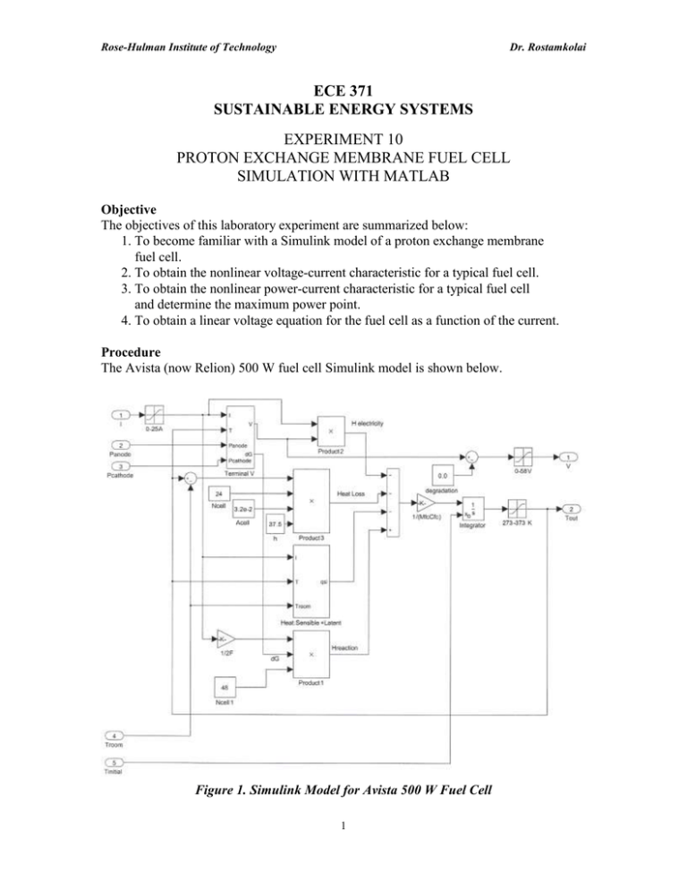
Rose-Hulman Institute of Technology
Dr. Rostamkolai
ECE 371
SUSTAINABLE ENERGY SYSTEMS
EXPERIMENT 10
PROTON EXCHANGE MEMBRANE FUEL CELL
SIMULATION WITH MATLAB
Objective
The objectives of this laboratory experiment are summarized below:
1. To become familiar with a Simulink model of a proton exchange membrane
fuel cell.
2. To obtain the nonlinear voltage-current characteristic for a typical fuel cell.
3. To obtain the nonlinear power-current characteristic for a typical fuel cell
and determine the maximum power point.
4. To obtain a linear voltage equation for the fuel cell as a function of the current.
Procedure
The Avista (now Relion) 500 W fuel cell Simulink model is shown below.
Figure 1. Simulink Model for Avista 500 W Fuel Cell
1
Rose-Hulman Institute of Technology
Dr. Rostamkolai
This model has 5 input and 2 output ports. The inputs consist of dc current, channel
pressure at the anode, channel pressure at the cathode, room temperature, and initial fuel
cell temperature. Outputs are output dc voltage, and fuel cell temperature. Multiplying the
dc voltage and current yields the dc power, which is an additional output quantity.
This fuel cell model will be modified to accomplish the objectives of this experiment.
The input current will be varied for a specified range. The other 4 inputs are constants.
The input current, output power, and output voltage are displayed on a Simulink XY
Graph. After you have verified that the simulation results are correct, you will pass each
of these to a workspace (simout) and plot the desirable graphs in Matlab.
Part 1 – Setting Up the Simulation
Obtain the proton exchange membrane Simulink model from your instructor’s website.
Double click on the Matlab icon on the desktop and then click on
Library Browser click on File  Open  PFMC_Sample.mdl
. In the Simulink
Next, modify the input ports for following conditions:
a. Choose a source for the current so you can linearly increase current from 0 to 25 A.
b. Choose a source for the channel pressure at the anode. This pressure will be
constant at 1.5 atm.
c. Choose a source for the channel pressure at the cathode. This pressure will be
constant at 1 atm.
d. Choose a source for the room temperature. This temperature will be constant at
34.5oC (convert it to Kelvin).
e. Choose a source for the initial temperature. This temperature will be constant at
34.5oC (convert it to Kelvin).
Then choose 2 channel scopes (XY Graph) to monitor the following input and outputs:
a. Input current as a function of time
b. Voltage as a function of current
c. Power as a function of current
Part 2 – Performing the Simulation
Perform the Simulink simulation by:
a. Clicking on Simulation button and choosing
Configuration Parameters
- Select the Simulation Start Time of 0.0 second
- Select the Simulation Stop Time of 25.1 seconds
- Select a Solver Option Type of “Fixed-Step”
and a Solver of “ode3”
- Select a Step Size of 0.01 second
- Click on OK
b. Running the simulation by clicking on the forward arrow
2
Rose-Hulman Institute of Technology
Dr. Rostamkolai
c. After completion of the simulation, check the results and make sure that they
make sense. The 3 oscilloscope (XY Graph) displays might be on top of each
other. If this is the case, move them around so you can see all 3 displays.
Part 3 – Plotting the Simulation Results
After you have confirmed that the simulation results are valid, pass on the dc current and
output variables to a sink called “Workspace”. Now the data is available in the Matlab
environment. Obtain and print a fine graph of the following by using the Matlab plot
command:
a. Input current as a function of time.
b. DC voltage as a function of the input current.
c. DC power as a function of the input current.
Part 4 – Determination of Values
Next determine the following values from Matlab plots (use the cursor button):
a. Fuel cell no-load voltage.
b. Fuel cell short-circuit current.
c. Fuel cell maximum power and the associated current.
Print the plots with the cursor values superimposed.
Part 5 – Linear Model Development
Linearize the V-I characteristic of the fuel cell that you obtained in Part 3, and write the
voltage equation. This can be done automatically with Matlab when you have the V-I
plot, and using a “Tool” called “Basic Fitting”.
Draw the circuit diagram of this linear device. Then create an Excel sheet and load this
device with resistances from 0.0 Ω to 200 Ω. Calculate the following:
a. Load current
b. Load Power
Now plot the load power as a function of the load current, and:
a. Visually compare this plot with the plot of Part 3.
b. Determine the resistance that yields the maximum power point.
c. Does this resistance validate the Maximum Power Transfer Theorem that you
learned in your Electric Circuit course?
d. Are the two resistances for maximum power transfer the same?
Documentation
At the end of the lab period, submit this document with your insertions, and:
 Matlab plot of the fuel cell input current as a function of time
 Matlab plot of fuel cell DC voltage as a function of the input current
 Matlab plot of fuel cell DC power as a function of the input current
 Matlab plot of the fuel cell linearized V-I trace superimposed on the nonlinear V-I
characteristic, and the equation for the straight line
 Excel plot of P as a function of I for the linearized model of the fuel cell
3