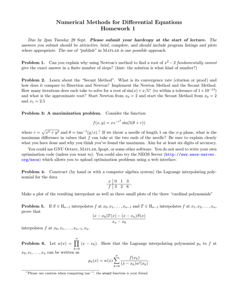
Numerical Methods for Differential Equations
Homework 1
Due by 2pm Tuesday 29 Sept. Please submit your hardcopy at the start of lecture. The
answers you submit should be attractive, brief, complete, and should include program listings and plots
where appropriate. The use of “publish” in Matlab is one possible approach.
Problem 1. Can you explain why using Newton’s method to find a root of x2 − 2 fundamentally cannot
give the exact answer in a finite number of steps? (hint: the solution is what kind of number?)
Problem 2. Learn about the “Secant Method”. What is its convergence rate (citation or proof) and
how does it compare to Bisection and Newton? Implement the Newton Method and the Secant Method.
How many iterations does each take to solve for a root of sin(x) + x/5? (to within a tolerance of 1 × 10−14 )
and what is the approximate root? Start Newton from x0 = 2 and start the Secant Method from x0 = 2
and x1 = 2.5
Problem 3: A maximization problem. Consider the function
2
f (x, y) = xe−r sin(5(θ + r))
p
where r = x2 + y 2 and θ = tan−1 (y/x).1 If we throw a needle of length 1 on the x-y plane, what is the
maximum difference in values that f can take at the two ends of the needle? Be sure to explain clearly
what you have done and why you think you’ve found the maximum. Aim for at least six digits of accuracy.
You could use GNU Octave, Matlab, Ipopt, or some other software. You do not need to write your own
optimization code (unless you want to). You could also try the NEOS Server (http://www.neos-server.
org/neos) which allows you to upload optimization problems using a web interface.
Problem 4. Construct (by hand or with a computer algebra system) the Lagrange interpolating polynomial for the data
x 0 1 3
.
f 3 2 6
Make a plot of the resulting interpolant as well as three small plots of the three “cardinal polynomials”
Problem 5.
prove that
If S ∈ Πn−1 interpolates f at x0 , x1 , . . . , xn−1 and T ∈ Πn−1 interpolates f at x1 , x2 , . . . , xn ,
(x − x0 )T (x) − (x − xn )S(x)
xn − x0
interpolates f at x0 , x1 , . . . , xn−1 , xn .
Problem 6.
Let w(x) =
n
Y
(x − xk ). Show that the Lagrange interpolating polynomial pn to f at
k=0
x0 , x1 , . . . , xn can be written as
pn (x) = w(x)
n
X
k=0
1
f (xk )
.
(x − xk )w0 (xk )
Please use caution when computing tan−1 : the atan2 function is your friend.
By dividing by a “clever form of 1”, derive the barycentric formula for Lagrange interpolation:
n
X
pn (x) =
k=0
wk
f (xk )
(x − xk )
n
X
k=0
where wk =
wk
(x − xk )
,
1
w0 (xk ) .
Problem 7. In the previous question, can you think of two things you might expect to go wrong when
implementing these formulae on a computer? Despite this, it turns out they are completely well-behaved
although this was only proven recently [Higham, The numerical stability of barycentric Lagrange interpolation, 2004], see also the survey article [Berrut & Trefethen, Barycentric Lagrange interpolation, 2004].
Write a software implementation of the barycentric formula for Lagrange interpolation. The inputs to
your function should be a vector of points (these are the nodes xk ) and another scalar x (the point at
which to interpolate). It should not take the f (xk ) as inputs. Your function should return the weights βk
so that
n
X
βk f (xk ).
pn (x) =
k=0
Use it to evaluate the interpolant of the data given in Problem 4 at x = 0.32, x = 2.999, and x = 1.
Display the resulting approximation to f (x) as well as the weights βk for each case, to at least 12 decimal
places.
Problem 8: Git (Mandatory for graduate students, optional for ugrads)
Create an account at github.com. Spend some time reading about “Git”. You may want to install
“SourceTree” or another app. On Mac/Linux you can also use command line tools.
Find instructor’s notes (written in a combination of Markdown and LATEX). Make a contribution to
the lecture notes and send a “pull request”. You may need to “fork” the repository. You may need to
“clone” it onto your local computer.
Some possible contributions:
• Fix a typo.
• Type a small part of a lecture (e.g., the “root finding” lecture notes are very sparse).
• Add a figure (ideally, in TikZ/PGF, but other formats ok).
• Something else. . .
(It should be a relatively small change: we want everyone to have a chance).
When preparing your HW hardcopy for submission, attach a screenshot showing your “pull request”
(something like github.com/.../pull/##). If it get merged before the assignment due date, great, but
don’t worry if it isn’t.