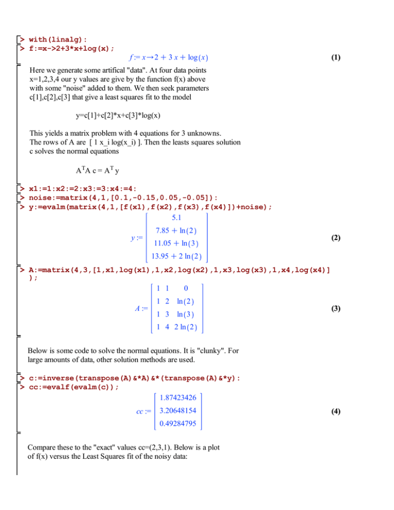
> with(linalg):
> f:=x->2+3*x+log(x);
f := x/2 C 3 x C log x
(1)
Here we generate some artifical "data". At four data points
x=1,2,3,4 our y values are give by the function f(x) above
with some "noise" added to them. We then seek parameters
c[1],c[2],c[3] that give a least squares fit to the model
y=c[1]+c[2]*x+c[3]*log(x)
This yields a matrix problem with 4 equations for 3 unknowns.
The rows of A are [ 1 x_i log(x_i) ]. Then the leasts squares solution
c solves the normal equations
ATA c = AT y
> x1:=1:x2:=2:x3:=3:x4:=4:
> noise:=matrix(4,1,[0.1,-0.15,0.05,-0.05]):
> y:=evalm(matrix(4,1,[f(x1),f(x2),f(x3),f(x4)])+noise);
5.1
y :=
7.85 C ln 2
11.05 C ln 3
(2)
13.95 C 2 ln 2
> A:=matrix(4,3,[1,x1,log(x1),1,x2,log(x2),1,x3,log(x3),1,x4,log(x4)]
);
1 1
0
A :=
1 2
ln 2
1 3
ln 3
(3)
1 4 2 ln 2
Below is some code to solve the normal equations. It is "clunky". For
large amounts of data, other solution methods are used.
> c:=inverse(transpose(A)&*A)&*(transpose(A)&*y):
> cc:=evalf(evalm(c));
1.87423426
cc :=
3.20648154
0.49284795
Compare these to the "exact" values cc=(2,3,1). Below is a plot
of f(x) versus the Least Squares fit of the noisy data:
(4)
> plot([f(x),cc[1,1]+cc[2,1]*x+cc[3,1]*log(x)],x=0..4);
15
10
5
0
1
2
x
K5
3
4