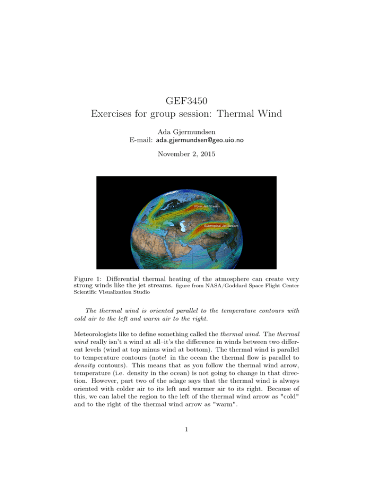
GEF3450
Exercises for group session: Thermal Wind
Ada Gjermundsen
E-mail: ada.gjermundsen@geo.uio.no
November 2, 2015
Figure 1: Differential thermal heating of the atmosphere can create very
strong winds like the jet streams. figure from NASA/Goddard Space Flight Center
Scientific Visualization Studio
The thermal wind is oriented parallel to the temperature contours with
cold air to the left and warm air to the right.
Meteorologists like to define something called the thermal wind. The thermal
wind really isn’t a wind at all–it’s the difference in winds between two different levels (wind at top minus wind at bottom). The thermal wind is parallel
to temperature contours (note! in the ocean the thermal flow is parallel to
density contours). This means that as you follow the thermal wind arrow,
temperature (i.e. density in the ocean) is not going to change in that direction. However, part two of the adage says that the thermal wind is always
oriented with colder air to its left and warmer air to its right. Because of
this, we can label the region to the left of the thermal wind arrow as "cold"
and to the right of the thermal wind arrow as "warm".
1
Figure 2: Ada’s handwavy sketch of thermal wind
This fancy feature of the thermal wind makes it useful for diagnosing temperature structures based on winds, or the other way around: calculate
wind profiles based on pressure or temperature measurements from different
heights in the atmosphere. It’s amazing how everything is connected!
Most of the text is taken from Luke’s weather blog: http://lukemweather.blogspot.no/
The Thermal Wind Balance:
There are several different versions of the thermal wind equation. For the atmosphere it is common to use the temperature gradient at constant pressure
surfaces to calculate the thermal wind
~ug
g
= − k̂ × ∇p T
(1)
∂p
fp
R p0
~uT = ~u(p1 ) − ~u(p0 ) = ln
]k̂ × ∇p T
(2)
f
p1
while in the ocean it is more common to consider changes in density (since
the thermal wind is parallel to density contours in the ocean)
~ug
g
=−
k̂ × ∇ρ
∂z
f ρc
... but don’t panic if you see other versions - they all describe the same
phenomenon:-)
2
(3)
Exercises:
Exercises from “Fluid Mechanics” by Kundu and Cohen, “Atmosphere, Ocean and Climate Dynamics” by Marshall and Plumb, “Atmospheric Science” by Wallace and Hobbs,
“Dynamic Meteorology" by Holton and “Geophysical Fluid Mechanics” by Weber.
1 The mean temperature in the layer between 750 hPa and 500 hPa decreases eastward by 3◦ C per 100 km. If the 750 hPa geostrophic wind
is from the southeast at 20 ms−1 , what is the geostrophic wind speed
and direction at 500 hPa? Let f = 10−4 s−1 .
2 What is the mean temperature advection in the 750 − 500 hPa layer
in problem 1?
3 Suppose that a vertical column of the atmosphere at 43◦ N is initially
isothermal from 900 hPa to 500 hPa. The geostrophic wind is 10 ms−1
from the south at 900 hPa, 10 ms−1 from the west at 700 hPa, and
20 ms−1 from the west at 500 hPa.
i) Calculate the mean horizontal temperature gradients in the two layers 900 hPa to 700 hPa and 700 hPa to 500 hPa.
(Hint: use the thermal wind eqn.)
ii) Compute the rate of advective temperature change in each layer.
(Hint: DT
Dt = 0 following the wind.)
iii) How long would this advection pattern have to persist in order to
establish a dry adiabatic lapse rate between 600 hPa and 800 hPa?
Assume that the lapse rate is constant between 900 hPa and 500 hPa,
and that the 600 hPa to 800 hPa thickness is 2.25 km?
(the dry adiabatic lapse rate is 9.8 ◦ Ckm−1 )
4 ) Fig 3 shows the trajectory of a “champion" surface drifter, which
made one and a half loops around Antarctica between March, 1995,
and March, 2000 (courtesy of Nikolai Maximenko). Red dots mark the
position of the float at 30 day interval.
i) Compute the speed of the drifter over the 5 years. (Hint: the distance for one loop around Antarctica at the latitude where the drifter
is located is approximately 22 × 103 km)
ii) Assuming that the mean zonal current at the bottom of the ocean
is zero, use the thermal wind relation (neglecting salinity effects) to
3
Figure 3: From “Atmosphere, Ocean and Climate Dynamics” by Marshall
and Plumb
compute the depth-averaged temperature gradient across the Antarctic Circumpolar Current (ACC). Hence estimate the mean temperature
drop across the 600 km-wide Drake Passage.
g ∂ρ
(Hint: use the thermal wind equation: f ∂u
∂z = ρref ∂y , the density equation for fresh water ρ = ρref (1−αT [T −Tref ]) where αT = 2×10−4 K−1
is the expansion coefficient and an average depth of 4 km)
iii) If the zonal current of the ACC increases linearly from zero at
the bottom of the ocean to a maximum at the surface (as measured
by the drifter), estimate the zonal transport of the ACC through
Drake Passage, assuming a meridional velocity profile as in Fig. 3
πy
(u(y, 0) = umax = U0 cos( 2L
)) and that the depth of the ocean is
4 km. The observed transport through Drake Passage is 130 SV. Is
your estimate roughly in accord? If not, why not?
5 ) Consider a straight, parallel, oceanic current at 45◦ N. For convenience, we define the x- and y- directions to along and across the
current, respectively. In the region −L < y < L, the flow velocity is
πy
z
) exp( )
2L
d
where z is height (note that z = 0 at mean sea level and decreases
u = U0 cos(
4
Figure 4: From “Atmosphere, Ocean and Climate Dynamics” by Marshall
and Plumb
downwards), L = 100 km, d = 400 m and U0 = 1.5 ms−1 . In the
region |y| > L, u = 0.The surface current is plotted in Fig 4. Using the
geostrophic, hydrostatic and thermal wind relations:
i) Determine and sketch the profile of surface elevation as a function
of y across the current.
ii) Determine and sketch the density difference, ρ(y, z) − ρ(0, z). (Hint:
g ∂ρ
use the thermal wind equation: f ∂u
∂z = ρref ∂y )
iii) Assuming the density is related to temperature by:
ρ = ρref (1 − αT [T − Tref ])
(4)
determine the temperature difference, T (L, z)−T (−L, z), as a function
of z. Use αT = 2 × 10−4 C−1 . Evaluate the difference at a depth of
500 m. Compare with Fig. 4.
6 Fig. 5 shows, schematically, the surface pressure contours (solid) and
mean 1000 hPa to 500 hPa temperature contours (dashed) in the vicinity of a typical northern hemisphere depression (storm). The contour
interval is 2 hPa for the surface pressure and 2◦ C for the temperature.
”L” indicates the low pressure center. Sketch the direction of the wind
near the surface, and on the 500 hPa pressure surface. (Assume that
the wind at 500 hPa is significantly larger than at the surface (why?).)
If the movement of the whole system is controlled by the 500 hPa wind,
how do you expect the storm to move? [Use: density of air at 1000 hPa
= 1.2 kgm−3 ; f = 7.27 × 10−5 s−1 ; gas constant for air = 287 Jkg−1 K.]
5
Figure 5: From “Atmosphere, Ocean and Climate Dynamics” by Marshall
and Plumb
7 i) From the pressure coordinate thermal wind relationship, (eqns. 3.4546 in the gfd notes), and approximating
∂u
∂u/∂z
'
∂p
∂p/∂z
(5)
show that in geometric height coordinates
∂u
g ∂T
'−
∂z
T ∂y
(6)
ii) The winter polar stratosphere is dominated by the “polar vortex”, a
strong westerly circulation about 60◦ latitude around the cold pole, as
depicted schematically in the Fig. 6. (This circulation is the subject of
considerable interest, because it is within the polar vortices - especially
that over Antarctica in the southern winter and spring - that most of
the ozone depletion is taking place.)
Assuming that the temperature at the pole is (at all heights) 50 K
colder at 80◦ latitude than at 40◦ latitude (and that it varies uniformly
in between), and that the westerly wind speed at 100 hPa pressure at
60◦ latitude is 10 ms−1 , use the thermal wind relation to estimate
the wind speed at 1 hPa pressure at 60◦ latitude. (you need the gas
constant for air = 287 Jkg−1 K).
6
Figure 6: From “Atmosphere, Ocean and Climate Dynamics” by Marshall
and Plumb
Solutions:
1 ~ug (500) = (−14.1, −20.4) ms−1 , or 25 ms−1 speed from 34◦ east of
north.
2 Mean advection = −~u · ∇T = −u ∂T
∂x , where u = (u500 − u750 )/2 and
∂T
−5◦
−1
Cm . Thus, = −~u · ∇T = −4.23 × 10−4◦ C s−1
∂x = −3 × 10
∂T
◦
3 For layer 900 − 700 hPa: ∂T
∂y = ∂x = −1.39 C/(100 km). The average
wind is u = v = 5 ms−1 .
∂T
◦
For layer 700 − 500 hPa: ∂T
∂y = −1.03 C/(100 km) and ∂x = 0.The
average wind is u = 15 ms−1 and v = 0 ms−1
∂T
∂T
The advective change of temperature change is ∂T
∂t = −u ∂x − v ∂y .
−4◦ C s−1 and for the
Thus for the 900 − 700 hPa layer ∂T
∂t = 1.39 × 10
700 − 500 hPa layer ∂T
∂t = 0. Thus, the temperature difference between
800 hPa and 600 hPa increases by 1.39 × 10−4◦ C s−1 . Assuming a
2.25 km thickness, we find that an adiabatic lapse rate (9.8◦ C/km)
would be established within 44 hrs.
4 i) u = 0.2 ms−1 .
ii) The depth average temperature drop is ∆T = 1.5 K
iii) 153 SV (observed transport is approx. 135 SV). Note that we have
only calculated the transport associated with the thermal wind.
5
6 The storm center should move approximately northeastwards at about
66 ms−1 .
7 ii) Given u100 = 10 ms−1 , we get u1 = 125 ms−1
7