Simple Random Sampling (Chapter 2)
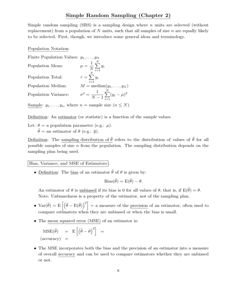
Simple random sampling (SRS) is a sampling design where n units are selected (without
replacement) from a population of N units, such that all samples of size n are equally likely
to be selected. First, though, we introduce some general ideas and terminology.
Population Notation:
Finite Population Values: y1 , . . . , yN
N
1 X
yi
Population Mean:
µ=
N i=1
Population Total:
τ=
N
X
yi
i=1
Population Median:
Population Variance:
M = median(y1 , . . . , yN )
N
1 X
σ2 =
(yi − µ)2
N − 1 i=1
Sample: y1 , . . . , yn , where n = sample size (n ≤ N ).
Definition: An estimator (or statistic) is a function of the sample values.
Let: θ = a population parameter (e.g.: µ).
θb = an estimator of θ (e.g.: y).
Definition: The sampling distribution of θb refers to the distribution of values of θb for all
possible samples of size n from the population. The sampling distribution depends on the
sampling plan being used.
Bias, Variance, and MSE of Estimators :
• Definition: The bias of an estimator θb of θ is given by:
b = E(θ)
b − θ.
Bias(θ)
b = θ.
An estimator of θ is unbiased if its bias is 0 for all values of θ, that is, if E(θ)
Note: Unbiasedness is a property of the estimator, not of the sampling plan.
b =E
• Var(θ)
·³
´2 ¸
b
b
θ − E(θ)
= a measure of the precision of an estimator, often used to
compare estimators when they are unbiased or when the bias is small.
• The mean squared error (MSE) of an estimator is:
b
MSE(θ)
= E
·³
´2 ¸
b
θ−θ
=
(accuracy) =
• The MSE incorporates both the bias and the precision of an estimator into a measure
of overall accuracy and can be used to compare estimators whether they are unbiased
or not.
8
• Many standard estimators are unbiased or nearly unbiased so the variance of estimators
is the most common means of comparison.
Example: Consider a population of size N = 4, with y1 = 6, y2 = 4, y3 = 16, & y4 = 10.
Population Mean µ = 36/4 = 9
i
1h
1
Population Variance σ 2 =
(6 − 9)2 + (4 − 9)2 + (16 − 9)2 + (10 − 9)2 = (84) = 28.
3
3
• Consider the following comparison of simple random sampling and stratified random
sampling for samples of size 2 from this population.
1. Take an SRS of size n = 2: Possible samples?
Sample
y
Prob.
We want to estimate µ with y.
1
54
(5 + · · · + 13) =
= 9, so y is an
6
6
unbiased estimator of µ.
1
1
42
Var(y) =
(5 − 9)2 + · · · + (13 − 9)2 =
= 7,
6
6
6
q
Var(y) = 2.65.
SD(y) =
E(y) =
2. Take a stratified random sample: Suppose we have 2 strata: 6, 4|16, 10. Does this seem
like a good choice of strata?
• Suppose we take a sample of size 1 from each stratum, and compute the stratified
estimator of the population mean: y s = 12 (y1 + y2 ). Possible Samples?
Sample
1
E(y s ) =
(11 + 8 + 10 + 7) = 9 (also unbiased for µ)
4
ys
Prob.
ys
5
7
11
13
Prob.
1/4
1/4
1/4
1/4
i
1h
(11 − 9)2 + · · · + (7 − 9)2 = 2.5
4
√
2.5 = 1.58.
SD(y s ) =
Var(y s ) =
• Since both estimators (SRS and stratified) are
unbiased, but y s has the smaller variance, a
stratified random sample is better here.
• Suppose instead that the 2 strata were defined as: 4, 16|6, 10.
Possible Samples
(4,6)
E(y s ) = 9, Var(y s ) = 10, and SD(y s ) = 3.16,
(4,10)
which is worse than the SRS in this case. Why?
(16,6)
(16,10)
9
– In the 1st set of strata, we have low
variability within strata (homogeneous within) & high variability between
strata (heterogeneous between).
– In the 2nd set of strata, we have high variability within strata (heterogeneous
within) & low variability between strata (homogeneous between).
– This example illustrates the importance of choosing strata which are heterogeneous between and homogeneous within. It should also serve as a warning
that stratification should not be used in sampling unless there are clear reasons
for believing the defined strata are quite different from one another. In other
words, don’t stratify without a good reason!
Back to Simple Random Sampling (N = population size, n = sample size)
Estimating the Mean
• We know that the population mean µ is estimated by y. What is the variance Var(y)?
• If N >> n, then the fpc ≈ 1 and is unnecessary. In this case, we revert to the usual
formula for the variance of the sample mean: Var(y) = σ 2 /n.
• If N = n (as in a census), then Var(y) =
• The derivation of the finite population corrected variance is somewhat tedious and is
covered on pages 21-22 of the text.
sµ
• The standard deviation of the sample mean is given by: SD(y) =
What is the problem with this as an estimator of variability?
¶
N − n σ2
.
N
n
• The population variance σ 2 is unknown, so we need to estimate it. This results in the
estimated standard deviation of y, more commonly referred to as the standard error of
y, given by:
s
d
SE(y) = SD(y)
=
µ
¶
n
N − n s2
1 X
where s2 =
(yi − y)2 .
N
n
n − 1 i=1
10
Estimating the Total : Estimate τ =
N
X
yi with τb =
i=1
n
NX
yi = N y .
n i=1
Var(τb) =
• In typical problems, we report the sample mean y & the standard error SE(y), and
form a confidence interval (CI) for µ as:



Critical   SE of
 =⇒ y ± t · SE(y) =⇒ y ± t ·
(Estimator) ± 
Value
Estimator
s
µ
¶
N − n s2
.
N
n
• Why is this interval t-based and not standard normal (z)-based?
• What assumptions are we are making in the use of this CI?
1.
2.
• If the first of these is violated, we can appeal to the Central Limit Theorem (CLT) to
obtain an approximate (1 − α) × 100% CI.
Usual Central Limit Theorem (CLT) : If y1 , . . . , yn are iid random variables with mean µ
·
and variance σ 2 < ∞, then: y ∼ N (µ, σ 2 /n) as n gets large.
• This version of the CLT is for an infinite population, where sampling with and without
replacement are the same.
Finite Population CLT: If y1 , . . . , yn are an SRS without replacement from a finite population, then:
!
Ã
µ
¶
N − n σ2
·
y ∼ N µ, Var(y) =
as both n and N − n get large.
N
n
Example: Suppose a study is undertaken to estimate the number of pellet groups for whitetailed deer in a 20-acre field. Sampling was done along 10 randomly located belt transects
of dimensions 3’x50’, where the number of pellet groups in each belt was counted.
• What is the sampling unit here?
• Suppose the following summary statistics were obtained: y = 5.55 groups, s2 = 14.06,
s = 3.75 groups, where:
µ = the mean number of pellet groups in a 3’x50’ transect,
τ = the total number of pellet groups in the 20 acres (1 acre = 43560 square feet).
11
• The goal here is to find an estimate τb of the total number of pellet groups using a
confidence interval. Computing:
y = 5.55 per 150 square feet =⇒ there are 5.55/150 pellet groups per square foot.
5.55
=⇒ τb =
·
43560
· |{z}
20 = 32234.4 groups,
| {z }


|150
{z }


# square feet  # acres

#
groups
per


per acre
square foot
=⇒ N =
43560 · 20
= 5808 (150 square foot areas in the 20-acre field).
150
• Note: This is not an infinite population because the transects have area; there are,
however, an infinite number of possible transects.
• The standard error of the sample mean number of groups per transect is:
s
µ
SE(y) =
n
1−
N
v
uµ
¶
u
10 14.06
u
=u 1−
= 1.186.
n
5808 } 10
t|
{z
¶ 2
s
.9983≈1
• This gives 95% confidence intervals for the mean and total as:
95% CI for µ :
y ± t.025 (9) · SE(y) = 5.55 ± 2.262(1.186) = (2.87, 8.23).
95% CI for τ :
(2.87 · 5808, 8.23 · 5808) = (16655, 47813).
Estimating Proportions (Ch. 5)


 1 if the ith unit has some characteristic 
. Define:
Let yi = 

0
otherwise
p =
N
1 X
yi = the population proportion of units with some characteristic,
N i=1
n
1X
yi = the sample proportion, with:
n i=1
N
p(1 − p) = the population variance,
=
N −1
n
b − p)
b = the sample variance.
=
p(1
n−1
pb =
σ2
s2
• Note that p & pb are defined exactly as µ & y were for these yi ’s. So, defined as above,
proportions can be represented as means.
The variance and estimated variance of pb follow immediately then from the forms of Var(y)
d
and Var(y)
given earlier in the handout:
µ
¶
µ
¶
µ
¶
N −n
N
N − n p(1 − p)
N − n σ2
=
p(1 − p) =
,
N
n
N
n(N − 1)
N −1
n
µ
¶
µ
¶
b − p)
b
N − n s2
N − n p(1
d p)
b =
Var(
=
.
N
n
N
n−1
b =
Var(p)
12
This estimated variance allows us to construct a confidence interval for p of the form:
v
Ã
!
u
u N − n p(1
b
b
−
p)
pb ± z t
.
N
n−1
• Is it valid to use such an interval? When?
• Exact confidence limits based on the hypergeometric distribution are given on page 41
of the text.
Design-Based vs. Model-Based Sampling: In everything we have looked at thus far, we have
taken a design-based or fixed-population approach to sampling. In other words, no distributional assumptions were placed on the data in finding the form of the estimators and their
variabilities. In the model-based approach to sampling, the “population” y1 , . . . , yN are considered to be random variables, that is, one possible realization of all possible realizations
that could have occurred under some model for the population.
For example, suppose I flip a (possibly biased) coin 100 times and record the result of
each toss on a slip of paper and place the slips in a box. I ask you, who don’t know the
results, to estimate the proportion of the 100 flips that came out heads. You are allowed to
take a sample of slips from which to make your estimate. This is a design-based approach –
the 100 flips is the population and the parameter of interest is the proportion of heads, say
θ, in these 100 flips. If you base your estimate on a random sample of slips of paper, the
only uncertainty in your estimate is due to sampling variability. If you could do a census,
there there would be no uncertainty in your estimate. If you use the the sample proportion
of heads as your estimator, then this estimator will be unbiased for θ and you will be able to
generate an unbiased estimate of its variance. These properties depend only on the sample
design – they don’t depend on whether I really flipped a coin 100 times or simply wrote
down 100 0’s and 1’s in any combination or order I wanted.
In the model based approach, we view these 100 flips as 100 realizations from a random
process, and the parameter we are really interested in is not the proportion of heads in these
100 flips, but the true long-term probability of heads. Our model might then be that the 100
flips are 100 independent Bernoulli trials with probability of heads p. Even if I observed all
100 flips, I would still not know p. The difference between the two approaches doesn’t really
make a difference in how I would estimate θ or p: I would use the proportion of heads in
whatever sample I observed. It would make a difference in the standard error of the estimate
as the population is considered infinite in the model based approach. It also has implications
for how I sample. If my model is correct – that these 100 flips are 100 independent Bernoulli
trials – then it doesn’t matter if I observe a random sample of flips or not. If I get to observe
10 flips, then the first 10 are just as good as any other set of 10. I simply view these 10
13
flips as 10 independent Bernoulli random variables; the randomness (and unbiasedness) in
my estimator comes from the model, not the sampling scheme. However, if my model is not
correct and these are not independent Bernoulli trials with constant probability of heads
(from example, there is dependence between trials, or the probability of heads decreases as
I go along), then my estimator based on the first 10 flips might not be very good (biased,
large variance) and I won’t realize it. In fact, the parameter p might not even make sense.
Design-based approaches are valid regardless of how the data were generated, but the scope
of inference is confined to the fixed population. The model-based approach allows for inference to a larger population or model, but depends crucially on the appropriateness of the
model.
14