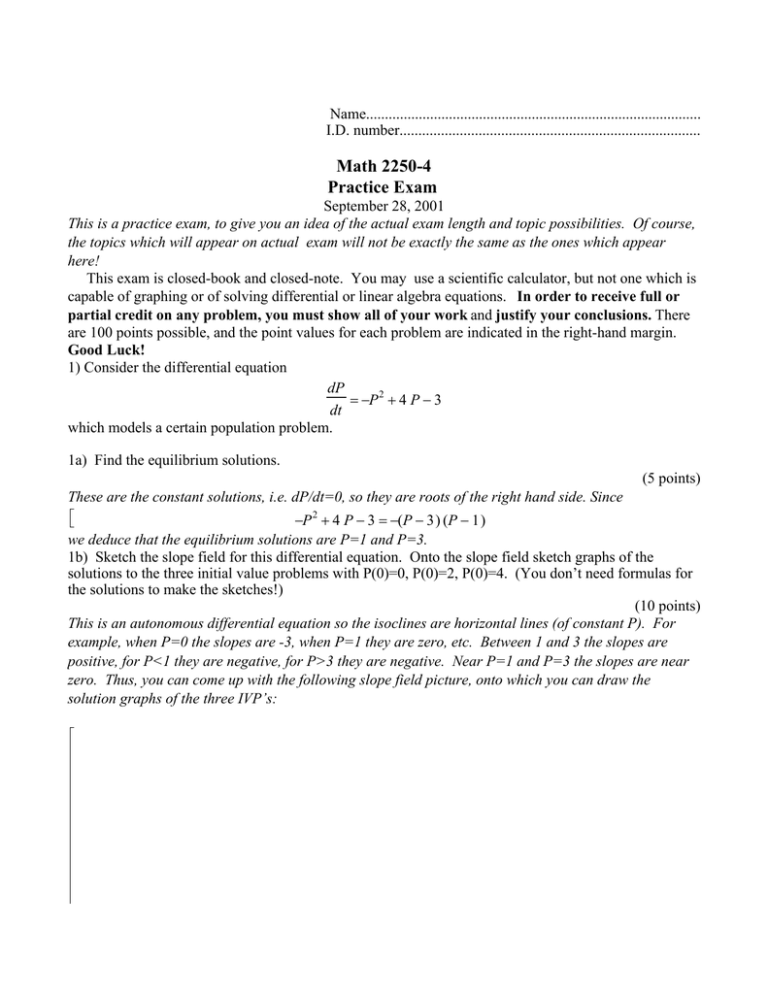
Name.........................................................................................
I.D. number................................................................................
Math 2250-4
Practice Exam
September 28, 2001
This is a practice exam, to give you an idea of the actual exam length and topic possibilities. Of course,
the topics which will appear on actual exam will not be exactly the same as the ones which appear
here!
This exam is closed-book and closed-note. You may use a scientific calculator, but not one which is
capable of graphing or of solving differential or linear algebra equations. In order to receive full or
partial credit on any problem, you must show all of your work and justify your conclusions. There
are 100 points possible, and the point values for each problem are indicated in the right-hand margin.
Good Luck!
1) Consider the differential equation
dP
2
= −P + 4 P − 3
dt
which models a certain population problem.
1a) Find the equilibrium solutions.
(5 points)
These are the constant solutions, i.e. dP/dt=0, so they are roots of the right hand side. Since
−P 2 + 4 P − 3 = −(P − 3 ) (P − 1 )
we deduce that the equilibrium solutions are P=1 and P=3.
1b) Sketch the slope field for this differential equation. Onto the slope field sketch graphs of the
solutions to the three initial value problems with P(0)=0, P(0)=2, P(0)=4. (You don’t need formulas for
the solutions to make the sketches!)
(10 points)
This is an autonomous differential equation so the isoclines are horizontal lines (of constant P). For
example, when P=0 the slopes are -3, when P=1 they are zero, etc. Between 1 and 3 the slopes are
positive, for P<1 they are negative, for P>3 they are negative. Near P=1 and P=3 the slopes are near
zero. Thus, you can come up with the following slope field picture, onto which you can draw the
solution graphs of the three IVP’s:
5
4
3
P(t)
2
1
–4
–2
0
–1
2
4
t
1c) Which of the equilibrium solutions are stable? Which are unstable?
(5 points)
We see that IVP’s with initial values near P=3 converge to P=3, so P=3 is asymptotically stable.
Solutions with IV’s near P=1 do not stay near P=1, so P=1 is unstable.
1d) Give a population model which leads to differential equations of this type. Be as precise as you can,
so that you can account for the signs of all three terms on the right-hand side of the differential equation.
(5 points)
An equation of the form
dP
= −P 2 + 4 P
dt
would be logistic, so what we have here is logistic, with constant rate harvesting.
1e) Find a explicit solution to the initial value problem for this differential equation, with P(0)=2. Verify
that your limiting population agrees with what your sketch predicted in part 1b).
(15 points)
We separate variables to solve this DE:
dP
= −dt
(P − 3 ) (P − 1 )
we use partial fractions to do the left-side integral:
1
A
B
+
=
(P − 3 ) (P − 1 ) P − 3 P − 1
1 = A (P − 1 ) + B (P − 3 )
letting P=1 and P=3 yields
1 = −2 B
1=2A
or
1
2
-1
B=
2
so, we multiply our separted DE by 2, and integrate:
ln( P − 3 ) − ln( P − 1 ) = −2 t + C
 P−3 
 = −2 t + C
ln
 P−1 
P−3
( −2 t )
=Ce
P−1
Since P(0)=2 we deduce
P−3
( −2 t )
= −e
P−1
A=
P − 3 = (1 − P ) e
P (e
( −2 t )
( −2 t )
+ 1) = 3 + e
P(t ) =
3+e
( −2 t )
( −2 t )
( −2 t )
+1
Thus P(t) --> 3 as t--> infinity.
2) Consider a brine tank which holds 15,000 gallons of continuously-mixed liquid. Let x(t) be the
amount of salt (in pounds) in the tank at time t. The in-flow and out-flow rates are both 150
gallons/hour, and the concentration of salt flowing in is 1 pound per 10 gallons of water.
2a) Explain how the information above leads to the differential equation
dx
+ .01 x = 15
dt
( 5 points)
The rate of change of x(t) is the rate at which salt is flowing in, minus the rate at which it is flowing out.
The rate at which it is flowing in is (0.1)*150 pounds/minute, and assuming uniform mixing the output
concentration is x/15,000 pounds/gallon, so the rate at which salt is flowing out is 150*x/15,000 = x/100
pounds per minute. Thus
dx
1
x
= 15 −
dt
100
which is equivalent to the given differential equation.
2b) Solve the initial value problem for this differential equation, assuming that at time t=0 there is no
salt in the water.
e
(10 points)
This is a linear DE, where "P(t)"=.01, so the integrating factor is exp(.01*t):

( .01 t )  dx
 + .01 x  = 15 e (.01 t )
e

 dt
integrate both sides to obtain
e
( .01 t )
x = 1500 e
( .01 t )
x(t ) = 1500 + C e
+C
( −.01 t )
Since x(0)=0 we deduce C=-1500, so
( −.01 t )
x(t ) = 1500 − 1500 e
2c) What is the limiting amount of salt as t approaches infinity?
(5 points)
The limiting amount of salt is 1500 pounds, which we expect since the limiting concentration should be
the concentration coming in, which is 0.1 pounds/gallon.
3) Consider the matrix
 2


A :=  1


 0
0
1
1
1


1


1
3a) Compute determinant(A). What does this computation tell you about whether A is singular or
nonsingular?
(5 points)
det(A)=2+0+1-0-2-0=1. Since det(A) is nonzero, the inverse of A exists.
3b) Find the inverse matrix to A, using the row-operation algorithm. Remember to show all work, as
always. Hint: The correct inverse matrix has no fractions in it, which you could deduce from your
answer to part (4a).
(15 points)
Augment A with the identity matrix and then compute the rref. Of course, on the exam you must do this
by hand and show your work. I’ll have maple do it:
 2 0 1 1 0 0




AaugId :=  1 1 1 0 1 0




 0 1 1 0 0 1
0
1 -1
1 0 0




2 -1
RREF :=  0 1 0 -1




1 -2
2
0 0 1
Thus the inverse matrix is
 0


 -1



 1
1
2
-2
-1


-1


2
3c) Recompute the inverse, using the adjoint formula. Show the cofactor matrix as well as the adjoint
matrix as intermediate steps, so that I can check your work.
(15 points)
The matrix of cofactors (equal to (-1)^(i+j) times the minor Mij) is
1
 0 -1





2 -2
cof :=  1




-1
-1
2


The adjoint is the transpose of the cofactor matrix:
1 -1
 0




2 -1
adj :=  -1




2
 1 -2
The inverse is 1/det times the adjoint matrix. Since det=1, the adjoint matrix above IS the inverse
matrix.
3d) Use the inverse matrix from (3b) or (3c) to solve the system
0
1  x   1
 2

 



 


  y  =  2
 1
1
1







 



 


1
1  z   2
 0
(5 points)
The solution to Ax=b is x=(inverse(A))*b:
 x


 y



 z
1
  0
 
 
 =  -1
2
 
 
 
  1 -2
 x  
 

 

 y =
 

 

 

z
 

(which is easily seen to solve the original system.)
-1 


-1 


2 
0


1


1
1


2


2