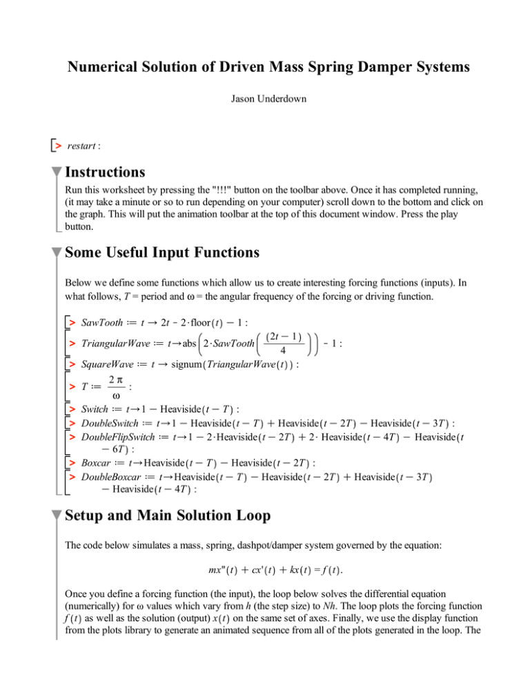
Numerical Solution of Driven Mass Spring Damper Systems
Jason Underdown
> restart :
Instructions
Run this worksheet by pressing the "!!!" button on the toolbar above. Once it has completed running,
(it may take a minute or so to run depending on your computer) scroll down to the bottom and click on
the graph. This will put the animation toolbar at the top of this document window. Press the play
button.
Some Useful Input Functions
Below we define some functions which allow us to create interesting forcing functions (inputs). In
what follows, T = period and w = the angular frequency of the forcing or driving function.
> SawTooth d t / 2t K2$floor t K 1 :
2t K 1
K1 :
4
SquareWave d t / signum TriangularWave t :
2p
Td
:
w
Switch d t/1 K Heaviside t K T :
DoubleSwitch d t/1 K Heaviside t K T C Heaviside t K 2T K Heaviside t K 3T :
DoubleFlipSwitch d t/1 K 2$Heaviside t K 2T C 2$ Heaviside t K 4T K Heaviside t
K 6T :
Boxcar d t/Heaviside t K T K Heaviside t K 2T :
DoubleBoxcar d t/Heaviside t K T K Heaviside t K 2T C Heaviside t K 3T
K Heaviside t K 4T :
> TriangularWave d t/abs 2$SawTooth
>
>
>
>
>
>
>
Setup and Main Solution Loop
The code below simulates a mass, spring, dashpot/damper system governed by the equation:
mx'' t C cx' t C kx t = f t .
Once you define a forcing function (the input), the loop below solves the differential equation
(numerically) for ω values which vary from h (the step size) to Nh. The loop plots the forcing function
f t as well as the solution (output) x t on the same set of axes. Finally, we use the display function
from the plots library to generate an animated sequence from all of the plots generated in the loop. The
animation shows how x t varies with the angular frequency of the forcing function, w.
Feel free to experiment with the code and change any of the values defined before the loop. Depending
on your computer's available memory, you probably don't want to set N any higher than about 500.
> m d 1 : c d 0 : k d 25 : Amp d 1 :
> solve m r2 C c r C k = 0, r # characteristic equation
2t
> f d t/Amp$SquareWave
:
T
> #fdt/Amp$cos w$t :
> #fdt/Amp$DoubleFlipSwitch t :
> IVs d x 0 = 0, x' 0 = 0 : # initial values
> tL d 30 : # t plot limit
> xL d 1.1$Amp : # x plot limit
> N d 100 : # number of frames in the animation
> h d .1 : # step size for incrementing w in the following loop
> for i from 1 to N do
w d i$h :
pin d plot f t , t = 0 ..tL, y =KxL ..xL, color = navy : # plot of forcing function f(t)
DE d m x'' t C c x' t C k x t = f t :
out d dsolve DE, IVs , x t , type = numeric :
pout d plots odeplot out, t, x t , t = 0 ..tL, numpoints = 600, view = 0 ..tL,KxL ..xL ,
caption = typeset "w= %1", w :
L i d plots display pin, pout : # combine plot of f(t) and x(t) into one plot
end do:
> plots display seq L i , i = 1 ..N , insequence = true