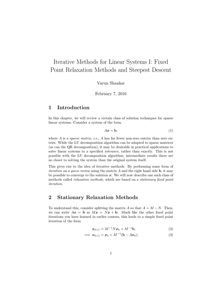
Iterative Methods for Linear Systems I: Fixed
Point Relaxation Methods and Steepest Descent
Varun Shankar
February 7, 2016
1
Introduction
In this chapter, we will review a certain class of solution techniques for sparse
linear systems. Consider a system of the form
Ax = b,
(1)
where A is a sparse matrix, i.e., A has far fewer non-zero entries than zero entries. While the LU decomposition algorithm can be adapted to sparse matrices
(as can the QR decomposition), it may be desirable in practical applications to
solve linear systems to a specified tolerance, rather than exactly. This is not
possible with the LU decomposition algorithm; intermediate results there are
no closer to solving the system than the original system itself.
This gives rise to the idea of iterative methods. By performing some form of
iteration on a guess vector using the matrix A and the right hand side b, it may
be possible to converge to the solution x. We will now describe one such class of
methods called relaxation methods, which are based on a stationary fixed point
iteration.
2
Stationary Relaxation Methods
To understand this, consider splitting the matrix A so that A = M − N . Then,
we can write Ax = b as M x = N x + b. Much like the other fixed point
iterations you have learned in earlier courses, this leads to a simple fixed point
iteration of the form
xk+1 = M −1 N xk + M −1 b,
=⇒ xk+1 = xk + M
1
−1
(b − Axk ).
(2)
(3)
Thus, beginning with a guess x0 , we iterate until xk+1 and xk are the same
(within some tolerance). Define the residual rk = b − Axk . Then, we have
xk+1 = xk + M −1 rk .
(4)
Clearly, the properties of M will dictate whether this iteration converges to x,
and at what rate. We will now discuss a few choices of the splitting matrix M .
The following methods are called stationary methods because the choice of M
is fixed over all iterations. Further, they are called relaxation methods because
they are all equivalent to a smoothing operation on the iterates xk .
How does one pick M ? Well, clearly, we want M −1 to be easy to compute (or
apply). At the same time, the best choice of M would be as close to A−1 as
possible. The tension between these two choices leads to different methods.
2.1
Jacobi iterations
In the Jacobi method, we pick M = D, where D is the diagonal matrix simply
containing the diagonal elements of A. With this choice, it is obviously trivially
easy to compute M −1 . Thus, we have
xk+1 = vxk + D−1 rk .
(5)
Notice that this never needs A supplied in explicit form. To get the residual, we
only need a routine that applies A to any vector (in this case, xk ). In component
form, the Jacobi iteration looks like this:


n
X
1 
aij xkj  , i = 1, . . . , n.
(6)
bi −
xk+1
=
i
aii
j=1,j6=i
For each component i, this iteration simply zeroes out the ith residual by adjusting xk . The other unknowns are not touched. Thus, each operation can be
performed on each unknown completely in parallel. While the Jacobi method is
not the fastest converging iterative method, its pleasingly parallel nature makes
it extremely popular in several contexts.
2.2
Gauss-Seidel
The Gauss-Seidel method involves picking M to be L, the lower triangular part
of A (including the diagonal). Since inverting a triangular system is in fact
fairly straightforward (forward substitution), the Gauss-Seidel method is only
slightly more expensive than the Jacobi method. More importantly, since we use
L rather than D, Gauss-Seidel converges twice as fast as Jacobi, when Jacobi
converges on the problem. The iteration is thus
xk+1 = xk + L−1 rk .
2
(7)
Remember: you should never explicitly form L−1 . Rather, you should perform
forward substitution to solve the system Ly = rk . In component form, GaussSeidel is given by


X
X
1 
xk+1
=
bi −
aij xk+1
−
aij xkj  , i = 1, . . . , n.
(8)
i
j
aii
j<i
j>i
Note that we use newly computed values xk+1
to compute other values xk+1
.
j
i
Thus, Gauss-Seidel cannot be executed straightforwardly in parallel.
2.3
Successive Over-Relaxation
The SOR method is straightforward. The idea is to use a combination of the
Jacobi idea and the Gauss-Seidel idea to improve on Gauss-Seidel’s convergence.
Thus, we say that
xk+1 ← ωxk+1 + (1 − ω)xk .
(9)
It can be shown that if 1 < ω < 2, the resulting algorithm (SOR) is much faster
than Gauss-Seidel. In matrix form, this is given by
xk+1 = xk + ω ((1 − ω)D + ωL)
−1
rk .
(10)
Typically, ω is chosen based on knowledge of the structure of A. For example,
if we know the eigenvalues of A in closed form, ω could be selected to be some
function of the eigenvalues of A.
2.4
Convergence of Stationary Relaxation Methods
We will now analyze the rate at which the above fixed point iterations converge
to the true solution. We know that the error at the k th step is
ek = x − xk = A−1 rk .
(11)
We want that as k → ∞, ek → 0. To derive the conditions for this, we must
analyze the properties of the iteration. Let us write the k th iterate as
xk = M −1 b + (I − M −1 A)xk−1 .
(12)
Formally, we also know that
x = M −1 b + (I − M −1 A)x.
(13)
Let T = I − M −1 A.Subtracting the two equations, we have
ek = T ek−1 = T (T ek−2 ) = . . . = T k e0 .
3
(14)
The matrix T is called the iteration matrix. Clearly, ek → 0 only if T k → 0.
This will happen if ||T || < 1 in any induced matrix norm.
It is also possible to derive a tighter bound. We in fact know that T k → 0 as
k → ∞ if the “magnitude” of T is less than 1. In other words, we simply want
the magnitude of the largest eigenvalue to be less than 1. This quantity (the
magnitude of the largest eigenvalue) is called the spectral radius of T , ρ(T ).
Thus, a fixed point iteration converges if ρ(T ) < 1. The rate of convergence, of
course, is determined by how small ρ(T ) is; the smaller the spectral radius, the
faster the convergence. Clearly, if the matrix T has large eigenvalues that are
somehow positive and greater than 1, the stationary iteration will not converge
unless the tolerance is chosen carefully.
3
Steepest Descent
In steepest descent, we now seek an iteration of the form
xk+1 = xk + αk pk ,
(15)
where pk is a search direction, and αk is a carefully-chosen constant (for each
iteration). Clearly, this is a generalization of the stationary methods discussed
thus far. The goal here is to pick pk = rk , and find the αk that helps us
“descend” fastest to the solution. Thus, we have an iteration of the form
xk+1 = xk + αk rk .
(16)
To find αk , we first remark that the solution x to any linear system of the form
Ax = b can be viewed as finding a vector x that minimizes
φ(x) =
1 T
x Ax − bT x.
2
(17)
To find αk , we similarly wish to minimize φ(xk + αrk ) over all values of α. This
amounts to minimizing
1
(xk + αrk )T A(xk + αrk ) − bT (xk + αrk ).
(18)
2
This is done by setting the derivative of the above function w.r.t α to 0. This
gives
φ(xk + αrk ) =
αrTk Ark + rTk Axk − rTk b = 0.
(19)
Using the fact that b − Ax = rk , we get
α = αk =
rTk rk
hrk , rk i
=
.
T
hrk , Ark i
rk Ark
(20)
Though the steepest descent method is typically faster than the relaxation
method, it displays the same order of convergence: the number of iterations
is linear in the number of unknowns. To get much faster convergence
4