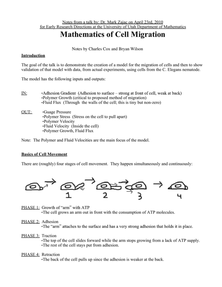
Notes from a talk by: Dr. Mark Zajac on April 23rd, 2010
for Early Research Directions at the University of Utah Department of Mathematics
Mathematics of Cell Migration
Notes by Charles Cox and Bryan Wilson
Introduction
The goal of the talk is to demonstrate the creation of a model for the migration of cells and then to show
validation of that model with data, from actual experiments, using cells from the C. Elegans nematode.
The model has the following inputs and outputs:
IN:
OUT:
Polymer Growth (critical to proposed method of migration)
Fluid Flux (Through the walls of the cell; this is tiny but non-zero)
Guage Pressure
Polymer Stress (Stress on the cell to pull apart)
Polymer Velocity
Fluid Velocity (Inside the cell)
Polymer Growth, Fluid Flux
Note: The Polymer and Fluid Velocities are the main focus of the model.
Basics of Cell Movement
There are (roughly) four stages of cell movement. They happen simultaneously and continuously:
PHASE 1:
The cell grows an arm out in front with the consumption of ATP molecules.
PHASE 2: Adhesion
PHASE 3: Traction
The top of the cell slides forward while the arm stops growing from a lack of ATP supply.
The rest of the cell stays put from adhesion.
PHASE 4: Retraction
The back of the cell pulls up since the adhesion is weaker at the back.
Method for Gathering Data
First we take microscopic digital video footage of a moving nematode by shining light through the semitransparent cell and measuring the phase difference in the light passing through it. The phase differential
We can track the movement speed within the cell by attempting to tell how far pixels in the picture move
per frame and dividing by the time between frames. If we know the size of one pixel in the image then
we know the speed it is moving.
The Problem: We would like this process to be computerized, but computers have trouble
integrate it, of course!
Integration of the phase difference gives a nice cell outline that a computer can handle.
We see from these experiments that cells tend to move faster as they are bigger, longer, and thinner. We
also see that the above inputs apparently do not tell the whole story, as the correlation between the data
and the mathematical model are very low.
Anisotropy
The cell has a cytoskeleton structure somewhat resembling a leaf, with ridges running from the back of
the cell toward the front. It would make sense to include something in the model which takes into
account compression forces pushing on the outside of the cell.
The front-back compression can be modeled as a very stiff spring (pushing directly against the hard
ridges) while the side-to-side compression is modeled as a series of springs, alternating stiff and weak
(ridges and fluids).
By including this in the model, we get better results. For graphs of cell shape vs. velocity we have:
(for best fit line to data) = 0.57
(for first attempt at model) = 0.25 (failure)
(for second attempt) = 0.52 (not great, but almost as good as the best fit line)
It is worth stressing that the data on these plots are highly scattered. Even the best fit line, while
statistically significant, is not visually compelling.
The Mathematics Behind the Model
Solid/Fluid Flow:
If is the percent volume of the cell taken by the cytoskeleton, then
percent volume taken by fluid.
is the
We assume that the drift/decay of the polymer is equivalent to its rigid translation.
We assume that the loss of polymer is equal to the gain in fluid.
Note that a 2-D model is justified because cells are very flat (and this is necessary to keep
the equations manageable).
Drag Force/Stress:
This force is on both the inside and the outside of the cell.
This is where the elasticity of the cell is important (Anisotropy).
Boundary Equations on the Cell:
the boundary of the cell may be rough. We solve the problem by smoothing things out with contours.
?
Create contour lines by solving differential equations
Use these contours to create normals from the cell edge
Use the normals to calculate curvature (for the boundary conditions)
The Equations in the Model
Translation: (Effective Outward Pressure) - (Inward Hydrostatic Pressure) = Bent Membrane
Counterbalance
Translation: Swept Volume = (Intracellular Flow) - (Transmembrane Flow)
Translation: Assembly Rate = Polymer Deficit and is positive
Conclusions / Remarks
The graphs of velocity vs. decay rate in the model fit the experimental data very well.
More pressure means less anisotropy is required for the model to be accurate.
Cytoskeletal decay can drive cell crawling.
Fluid (Cytosolic) effects are important.
It is important not to neglect the membrane permeability.