Math 5010 § 1.
Treibergs
Solutions to Seventh Homework
March 6, 2009
151[25] Suppose that the probability of an insect laying n eggs is given by the Poisson distribution
with mean µ > 0, that is, by the probability distribution given over all the nonnegative integers defined by e−µ µn /n!, n ∈ D = {0, 1, 2, 3, . . .}. Suppose further, that the probability of
an egg developing is p. Assuming mutual independence of the eggs, show that the probability
distribution fY (y) for the probability that there are y survivors is also of Poisson type, and
find the mean.
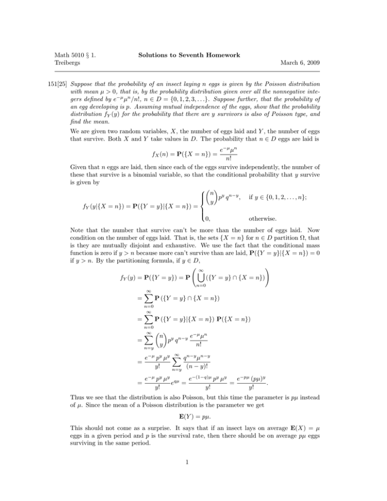
We are given two random variables, X, the number of eggs laid and Y , the number of eggs
that survive. Both X and Y take values in D. The probability that n ∈ D eggs are laid is
e−µ µn
n!
Given that n eggs are laid, then since each of the eggs survive independently, the number of
these that survive is a binomial variable, so that the conditional probability that y survive
is given by
 n y n−y


, if y ∈ {0, 1, 2, . . . , n};
 y p q
fY (y|{X = n}) = P({Y = y}|{X = n}) =



0,
otherwise.
fX (n) = P({X = n}) =
Note that the number that survive can’t be more than the number of eggs laid. Now
condition on the number of eggs laid. That is, the sets {X = n} for n ∈ D partition Ω, that
is they are mutually disjoint and exhaustive. We use the fact that the conditional mass
function is zero if y > n because more can’t survive than are laid, P({Y = y}|{X = n}) = 0
if y > n. By the partitioning formula, if y ∈ D,
!
∞
[
fY (y) = P({Y = y}) = P
({Y = y} ∩ {X = n})
n=0
=
=
=
∞
X
n=0
∞
X
P ({Y = y} ∩ {X = n})
P ({Y = y}|{X = n}) P({X = n})
n=0
∞ X
n=y
n y n−y e−µ µn
p q
y
n!
=
∞
e−µ py µy X q n−y µn−y
y!
(n − y)!
n=y
=
e−µ py µy qµ
e−(1−q)µ py µy
e−pµ (pµ)y
e =
=
.
y!
y!
y!
Thus we see that the distribution is also Poisson, but this time the parameter is pµ instead
of µ. Since the mean of a Poisson distribution is the parameter we get
E(Y ) = pµ.
This should not come as a surprise. It says that if an insect lays on average E(X) = µ
eggs in a given period and p is the survival rate, then there should be on average pµ eggs
surviving in the same period.
1
[A.] Suppose that X ∼ Geom(p) is a geometric random variable with parameter p. Find
(a) P(X is odd);
(b) P(X is even);
(c) P(X > k);
(d) Let k be an integer such that 1 ≤ k ≤ n. Find P(X = k|X ≤ k);
(e) P(2 ≤ X ≤ 9|X ≥ 4);
(f ) Let k ∈ N. Let g(x) = min(x, k) and Y = g(X). Find the pmf fY (y) and the
expectation E(Y );
(g) E(1/X).
The standard picture of a geometric variable is a sequence of independent coin flips where
the probability of head is p and X is the number of flips to get the first head. It takes
values in the natural numbers D = N = {1, 2, 3, . . .}, and its pmf for x ∈ D is
fX (x) = P(X = x) = p q x−1 .
(a.) The event that X is odd is given by
{X is odd} = {X = 1} ∪ {X = 3} ∪ {X = 5} ∪ · · · =
∞
[
{X = 2k + 1}
k=0
Since these are disjoint events, we may add using the geometric sum
with r = q 2 ,
P(X is odd) =
∞
X
P(X = 2k + 1) =
k=0
∞
X
k=0
p q 2k =
P∞
k=0
rk = (1 − r)−1
1
p
=
.
2
1−q
1+q
(b.) The complementary event is
P(X is even) = P({X is odd}c ) = 1 − P(X is odd) = 1 −
1
q
=
.
1+q
1+q
(c.) The event that X is greater than k is
[
{X > k} =
{X = x}
x ∈ D and x > k
Since these are disjoint events, we may add using the geometric sum. If k + 1 ∈ D,
P(X > k) =
∞
X
p q x−1 = p q k + q k+1 + q k+2 + · · ·
x=k+1
p qk
= p qk 1 + q + q2 + · · · =
= qk .
1−q
Note that this implies for k ∈ D, P(X ≥ k) = P(X > k − 1) = q k−1 . Also the cumulative
distribution function for x ∈ D,
FX (x) = P(X ≤ x) = P({X > x}c ) = 1 − P(X > x) = 1 − q x .
2
(1)
(d.) If k is an integer so that 1 ≤ k ≤ n, then the event
{X = k} ⊂ {X ≤ n}.
Compute conditional probabilities as usual using (1)
P(X = k|X ≤ n) =
P({X = k} ∩ {X ≤ n})
P(X = k)
p q k−1
.
=
=
P(X ≤ n)
P(X ≤ n)
1 − qn
(e.) Using the fact that the latter events are disjoint
{X > 3} = {4 ≤ X ≤ 9} ∪ {X > 9}
we get the probability using (c.),
P(4 ≤ X ≤ 9) = P(X > 3) − P(X > 9) = q 3 − q 9 .
Equivalently, P(4 ≤ X ≤ 9) = P(X ≤ 9) − P(X ≤ 3) = FX (9) − FX (3). We compute
conditional probabilities as usual:
P(2 ≤ X ≤ 9|X ≥ 4) =
P({2 ≤ X ≤ 9} ∩ {X ≥ 4})
P(4 ≤ X ≤ 9)
q3 − q9
=
=
= 1 − q6 .
P(X ≥ 4)
P(X > 3)
q3
(f.) For the natural number k, the function
(
x,
g(x) = min(x, k) =
k,
if x < k;
if x ≥ k.
g maps D to D0 = {1, 2, 3, . . . , k}. Thus if y ∈ D0 and y < k then there is exactly one
x ∈ D such that y = g(x), namely, x = y. If y = k then the set of x’s that map to k is
{k, k + 1, k + 2, . . .} = {X ≥ k}. This set is also called the preimage g −1 ({k}). Using the
formula for the pmf of the new random variable Y = g(X) we have
X
fY (y) =
fX (x).
x ∈ D such that g(x) = y
For this g(X), using (c.), it becomes for y ∈ D0 ,
(
fX (y) = p q y−1 ,
if y < k;
fY (y) = P∞
k−1
f
(x)
=
P(X
≥
k)
=
q
,
if x = k.
x=k X
Of course, fY (y) = 0 if y ∈
/ D0 .
To find the expectation we may use the definition or Theorem 4.3.4, which give the same
expression. Thus if k > 1,
!
!
k−1
k−1
X
X
X
d
E(Y ) =
y fY (y) =
y p q y−1 + kq k−1 = p
q y + kq k−1
dq
0
y=1
y=0
y∈D
k−1
k
d 1 − qk
−kq
1
−
q
1 − qk
+ kq k−1 = p
+ kq k−1 =
=p
+
.
2
dq 1 − q
1−q
(1 − q)
p
If k = 1 there is one term and E(Y ) = 1 so the formula works for k ≥ 1 as well. Since
g(x) ≤ x, it is no surprise that this is close to but less than E(X) = 1/p.
(g.) To find the expectation of Z = h(X) where h(x) = 1/x, we use Theorem 4.3.4.
E(Z) =
X
x∈D
h(x) fX (x) =
∞
X
p q x−1
x=1
x
See problem 151[18] and page 23.
3
∞
=
p X qx
p log(1 − q)
p log p
=−
=−
.
q x=1 x
q
q
[B.] Suppose that an unfair coin is tossed repeatedly. Suppose that the tosses are independent
and the probability of each head is p. Let X denote the number of tosses it takes to get three
heads. Derive the formulas for E(X) and Var(X).
X is distributed according to the negative binomial distribution with parameters k = 3 and
p. The variable takes values in D = {k, k + 1, k + 2, . . .} since one must toss the coin k times
at least in order to have k heads. In order that the k-th head occur at the x-th toss, there
must be k − 1 heads in the first x − 1 tosses and the x-th toss has to be a head. Thus the
negative binomial pmf is for x ∈ D,
x − 1 k x−k
fX (x) =
p q
.
k−1
The expectation is given by the sum
X
E(X) =
x∈D
∞
X
x − 1 k x−k
x fX (x) =
x
p q
.
k−1
x=k
Using the formula for binomial coefficients,
x
k x!
k x!
x−1
x (x − 1)!
=
=
=k
.
x
=
x−k
(k − 1)! (x − k)!
k (k − 1)! (x − k)!
k! (x − k)!
k−1
Inserting and changing dummy index by j = x − k,
∞
∞ X
X
x
k+j j
E(X) =
k
pk q x−k = k pk
q .
x−k
j
j=0
x=k
From page 22, the negative binomial series is
∞ X
m+j−1 j
z = (1 − z)−m
j
j=0
which makes sense even if m > 0 is a real number. In our series, the role of m is played by
m = k + 1. Thus
k
E(X) = k pk (1 − q)−(k+1) = .
p
To compute the variance, we use the computation formula
Var(X) = E(X 2 ) − E(X)2 .
Using the equation x2 = (x + 1)x − x, the expectation of the square is
∞
X
X
2
2
2 x−1
E(X ) =
x fX (x) =
x
pk q x−k
k−1
x∈D
x=k
∞
∞
X
x − 1 k x−k X
x − 1 k x−k
=
(x + 1)x
p q
−
x
p q
.
k−1
k−1
x=k
x=k
The second sum is − E(X). We have another binomial coefficient identity
x−1
(x + 1) x (x − 1)!
(k + 1) k (x + 1)!
(x + 1)x
=
=
k−1
(k − 1)! (x − k)!
(k + 1) k (k − 1)! (x − k)!
(k + 1) k (x + 1)!
x+1
=
= (k + 1)k
.
(k + 1)! (x − k)!
x−k
4
Inserting this, changing dummy index to j = x − k and using m = k + 2 in the negative
binomial series, the first sum in E(X 2 ) yields
∞
X
∞
x − 1 k x−k X
x + 1 k x−k
(x + 1)x
p q
=
(k + 1)k
p q
k−1
x−k
x=k
x=k
∞ X
k+j+1 j
(k + 1)k
k
.
= (k + 1)kp
q = (k + 1)kpk (1 − q)−(k+2) =
p2
j
j=0
Assembling,
Var(X) =
(k + 1)k − pk − k 2
kq
(k + 1)k k k 2
−
=
= 2.
−
2
2
2
p
p
p
p
p
5