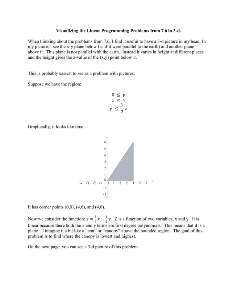
Visualizing the Linear Programming Problems from 7.6 in 3-d.
When thinking about the problems from 7.6, I find it useful to have a 3-d picture in my head. In
my picture, I see the x-y plane below (as if it were parallel to the earth) and another plane –
above it. This plane is not parallel with the earth. Instead it varies in height at different places
and the height gives the z-value of the (x,y) point below it.
This is probably easiest to see as a problem with pictures:
Suppose we have the region:
Graphically, it looks like this:
It has corner points (0,0), (4,6), and (4,0).
Now we consider the function:
. Z is a function of two variables, x and y. It is
linear because there both the x and y terms are first degree polynomials. This means that it is a
plane. I imagine it a bit like a “tent” or “canopy” above the bounded region. The goal of this
problem is to find where the canopy is lowest and highest.
On the next page, you can see a 3-d picture of this problem.
This link lets you model linear programming problems in 3-d. It took me a few minutes to figure
out how to change the equations, but once I got the hang of it, I really appreciated “seeing” the
picture behind the problem.
http://www.teacherlink.org/content/math/interactive/flash/linearprogramming/linearprogrammin
g.html