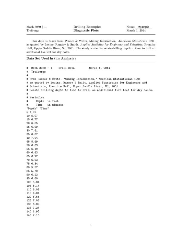
Math 3080 § 1.
Treibergs
Drilling Example:
Diagnostic Plots
Name: Example
March 1, 2014
This data is taken from Penner & Watts, Mining Information, American Statistician 1991,
as quoted by Levine, Ramsey & Smidt, Applied Statistics for Engineers and Scientists, Prentice
Hall, Upper Saddle River, NJ, 2001. The study wished to relate drilling depth to time to drill an
additional five feet for dry holes.
Data Set Used in this Analysis :
# Math 3080 - 1
Drill Data
March 1, 2014
# Treibergs
#
# From Penner & Watts, "Mining Information," American Statistician 1991
# as quoted by levine, Ramsey & Smidt, Applied Statistics for Engineers and
# Scientists, Prentice Hall, Upper Saddle River, NJ, 2001.
# Relate drilling depth to time to drill an additional five feet for dry holes.
#
# Variables
#
Depth in feet
#
Time
in minutes
"Depth" "Time"
5 4.90
10 5.07
15 6.77
20 6.65
25 6.99
30 7.41
35 6.07
40 7.04
45 5.49
50 6.03
55 6.19
60 6.43
65 6.27
70 6.03
75 6.34
80 5.57
85 5.70
90 6.23
95 6.60
100 5.84
105 5.17
110 6.03
115 6.84
120 6.58
125 7.03
130 6.89
135 7.27
140 6.92
145 7.15
1
150
155
160
165
170
175
180
185
190
195
200
205
210
215
220
225
230
235
240
245
250
7.25
7.05
6.95
6.76
5.97
7.75
7.11
7.07
7.17
6.91
6.15
6.19
6.29
5.58
7.22
7.62
8.28
7.59
6.42
7.12
6.62
R Session:
R version 2.10.1 (2009-12-14)
Copyright (C) 2009 The R Foundation for Statistical Computing
ISBN 3-900051-07-0
R is free software and comes with ABSOLUTELY NO WARRANTY.
You are welcome to redistribute it under certain conditions.
Type ’license()’ or ’licence()’ for distribution details.
Natural language support but running in an English locale
R is a collaborative project with many contributors.
Type ’contributors()’ for more information and
’citation()’ on how to cite R or R packages in publications.
Type ’demo()’ for some demos, ’help()’ for on-line help, or
’help.start()’ for an HTML browser interface to help.
Type ’q()’ to quit R.
[R.app GUI 1.31 (5538) powerpc-apple-darwin8.11.1]
[Workspace restored from /Users/andrejstreibergs/.RData]
> tt = read.table("M3082DataDrill.txt",header=T)
> attach(tt)
2
> tt
Depth
1
5
2
10
3
15
4
20
5
25
6
30
7
35
8
40
9
45
10
50
11
55
12
60
13
65
14
70
15
75
16
80
17
85
18
90
19
95
20
100
21
105
22
110
23
115
24
120
25
125
26
130
27
135
28
140
29
145
30
150
31
155
32
160
33
165
34
170
35
175
36
180
37
185
38
190
39
195
40
200
41
205
42
210
43
215
44
220
45
225
46
230
47
235
48
240
49
245
50
250
Time
4.90
5.07
6.77
6.65
6.99
7.41
6.07
7.04
5.49
6.03
6.19
6.43
6.27
6.03
6.34
5.57
5.70
6.23
6.60
5.84
5.17
6.03
6.84
6.58
7.03
6.89
7.27
6.92
7.15
7.25
7.05
6.95
6.76
5.97
7.75
7.11
7.07
7.17
6.91
6.15
6.19
6.29
5.58
7.22
7.62
8.28
7.59
6.42
7.12
6.62
3
> names(tt)
[1] "Depth" "Time"
> ############# SCATTERPLOT OF DATA WITH REGRESSION LINE ############
> plot(Time~Depth,
main = "Scatter Plot of Drilling Depth v. Time to Drill next 5’")
> f1 = lm(Time~Depth); abline(f1,col=2)
> # M3082Drill1.pdf
>
> ############### PLOT STD. RESID. VS X ############################
>
> plot(rstandard(f1)~Depth,ylab="Standardized Residuals of Time",
main="Std. Resid. of Time vs. Depth",ylim=max(abs(rstandard(f1)))*c(-1,1))
> abline(h=c(0,2,-2),lty=c(5,2,2))
>
> ############### PLOT STD. RESID. VS FITTED #######################
>
> plot(rstandard(f1)~fitted(f1), ylab="Standardized Residuals of Time",
xlab="Fitted Values",main="Std. Resid. of Time vs. Fitted Values",
ylim=max(abs(rstandard(f1)))*c(-1,1))
> abline(h=c(0,2,-2),lty=c(5,2,2))
>
> ############### PLOT FITTED VS OBSERVED ##########################
>
> plot(fitted(f1)~Time, ylab="Fitted values of Time",
xlab = "Observed Time Values",
main = "Fitted Values of Time vs. Observed Values of Time",
xlim = c(mi,ma), ylim = c(mi,ma))
>
> ############### NORMAL Q-Q PLOT OF STD. RESID.#####################
>
> qqnorm(rstandard(f1), ylab = "Standardized Residuals of Time",
main = "QQ-Plot of Std. Resid. of Time",
ylim = max(abs(rstandard(f1)))*c(-1,1))
> abline(h=c(0,2,-2), lty=c(5,2,2)); abline(0,1,col=2)
>
> ########### PLOT STANDARDIZED RESIDUALS VS INDEX: DATA ORDER ######
>
> plot(rstandard(f1), ylab = "Standardized Residuals of Time",
xlab = "i = order of observation",
main = "Std. Resid. of Time vs. i = Order of Observation",
ylim = max(abs(rstandard(f1)))*c(-1,1))
> abline(h=c(0,2,-2),lty=c(5,2,2))
>
> ################# CANNED DIAGNOSTIC PLOTS #########################
>
> layout(matrix(c(1,3,2,4),nrow=2))
> plot(f1)
> # M3082Drill7.pdf
4
> ################### SUMMARY AND ANOVA TABLE FOR REGRESSION
>
> summary(f1); anova(f1)
######
Call:
lm(formula = Time ~ Depth)
Residuals:
Min
1Q
-1.38156 -0.58099
Median
0.03983
3Q
0.44131
Max
1.27335
Coefficients:
Estimate Std. Error t value Pr(>|t|)
(Intercept) 6.002882
0.186050 32.265 < 2e-16 ***
Depth
0.004459
0.001270
3.511 0.000982 ***
--Signif. codes: 0 *** 0.001 ** 0.01 * 0.05 . 0.1
1
Residual standard error: 0.6479 on 48 degrees of freedom
Multiple R-squared: 0.2043,Adjusted R-squared: 0.1878
F-statistic: 12.33 on 1 and 48 DF, p-value: 0.0009821
Analysis of Variance Table
Response: Time
Df Sum Sq Mean Sq F value
Pr(>F)
Depth
1 5.1756 5.1756 12.328 0.0009821 ***
Residuals 48 20.1520 0.4198
--Signif. codes: 0 *** 0.001 ** 0.01 * 0.05 . 0.1
1
>
> ############## SHAPIRO WILK TEST FOR NORMALITY ###################
>
> shapiro.test(rstandard(f1))
Shapiro-Wilk normality test
data: rstandard(f1)
W = 0.977, p-value = 0.4323
>
>
>
5
6.5
6.0
5.5
5.0
Time
7.0
7.5
8.0
Scatter Plot of Drilling Depth v. Time to Drill next 5'
0
50
100
150
Depth
6
200
250
1
0
-1
-2
Standardized Residuals of Time
2
Std. Resid. of Time vs. Depth
0
50
100
150
Depth
7
200
250
1
0
-1
-2
Standardized Residuals of Time
2
Std. Resid. of Time vs. Fitted Values
6.0
6.2
6.4
6.6
Fitted Values
8
6.8
7.0
7.0
6.5
6.0
5.5
5.0
Fitted values of Time
7.5
8.0
Fitted Values of Time vs. Observed Values of Time
5.0
5.5
6.0
6.5
7.0
Observed Time Values
9
7.5
8.0
1
0
-1
-2
Standardized Residuals of Time
2
QQ-Plot of Std. Resid. of Time
-2
-1
0
Theoretical Quantiles
10
1
2
1
0
-1
-2
Standardized Residuals of Time
2
Std. Resid. of Time vs. i = Order of Observation
0
10
20
30
i = order of observation
11
40
50
Normal Q-Q
6.2
6.4
6.6
6.8
1
0
-2
43
-1
Standardized residuals
0.5
-0.5
21
6.0
6
2
6
-1.5
Residuals
1.5
Residuals vs Fitted
7.0
43
-2
Fitted values
2
1
0
-1
Standardized residuals
2
46
1
-2
1.5
1.0
Standardized residuals
21
6.4
1
Residuals vs Leverage
0.5
6.2
0
43
Cook's distance
0.0
6.0
-1
Theoretical Quantiles
Scale-Location
6
21
6.6
6.8
7.0
0.00
Fitted values
0.02
0.04
Leverage
12
43
0.06
0.08