Math 3080 § 1.
Treibergs
Tea Data: Unbalanced Design in
Single Factor ANOVA
Data File Used in this Analysis:
Name: Example
March 15, 2010
6.6
1
9.8
2
5.0
3
7.9
4
8.6
1
6.1
2
7.4
3
4.5
4
8.9
1
8.4
2
5.3
3
5.0
4
10.1
1
6.1
3
9.6
1
4.0
4
# M3080 - 1
#
Tea Data March 17 2010
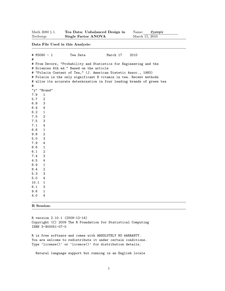
# From Devore, "Probability and Statistics for Engineering and the
# Sciences 4th ed." Based on the article
# "Folacin Content of Tea," (J. American Dietetic Assoc., 1983)
# Folacin is the only significant B vitamin in tea. Recent methods
# allow its accurate determination in four leading brands of green tea
#
"y" "Brand"
7.9
1
5.7
2
6.8
3
6.4
4
6.2
1
7.5
2
7.5
3
7.1
4
R Session:
R version 2.10.1 (2009-12-14)
Copyright (C) 2009 The R Foundation for Statistical Computing
ISBN 3-900051-07-0
R is free software and comes with ABSOLUTELY NO WARRANTY.
You are welcome to redistribute it under certain conditions.
Type ’license()’ or ’licence()’ for distribution details.
Natural language support but running in an English locale
1

R is a collaborative project with many contributors.
Type ’contributors()’ for more information and
’citation()’ on how to cite R or R packages in publications.
Type ’demo()’ for some demos, ’help()’ for on-line help, or
’help.start()’ for an HTML browser interface to help.
Type ’q()’ to quit R.
[R.app GUI 1.31 (5538) powerpc-apple-darwin8.11.1]
[Workspace restored from /Users/andrejstreibergs/.RData]
> tt <- read.table("M3081DataTea.txt", header=TRUE)
> tt y Brand
1 7.9
1
2 5.7
3 6.8
2
3
4 6.4
5 6.2
6 7.5
7 7.5
4
1
2
3
8 7.1
9 6.6
10 9.8
11 5.0
12 7.9
13 8.6
14 6.1
15 7.4
16 4.5
17 8.9
18 8.4
4
1
2
3
4
1
2
3
4
1
2
19 5.3
20 5.0
21 10.1
22 6.1
1
3
3
4
23 9.6
24 4.0
1
4
> attach(tt)
> brand <- factor(Brand)
>#=====================SUMMARY STATS FOR EACH BRAND=======
> tapply(y,brand,summary)
$‘1‘
Min. 1st Qu.
Median Mean 3rd Qu.
Max.
6.200
7.250
8.600
8.271
9.250
10.100
$‘2‘
Min. 1st Qu.
Median
5.7
6.1
7.5
Mean 3rd Qu.
7.5
8.4
Max.
9.8
$‘3‘
2

Min. 1st Qu.
Median
5.00
5.50
6.45
Mean 3rd Qu.
6.35
7.25
Max.
7.50
$‘4‘
Min. 1st Qu.
Median Mean 3rd Qu.
Max.
4.000
4.625
5.700
5.817
6.925
7.900
>#============================ANALYSIS OF VARIANCE============
> f1<-aov(y~brand);summary(f1) brand
Df Sum Sq Mean Sq F value Pr(>F)
3 23.496
7.8319
Residuals 20 41.778
2.0889
3.7493 0.02755 *
---
Signif. codes: 0 *** 0.001 ** 0.01 * 0.05 . 0.1
1
>#=============DISPLAY MEANS (MU, MU_i’S AND J_i’S)============
> model.tables(f1, type="means")
Tables of means
Grand mean
7.016667
brand
1 2 3 4
8.271 7.5 6.35 5.817
rep 7.000 5.0 6.00 6.000
>#=========================DISPLAY EFFECTS (ALPHA_i’S)=========
> model.tables(f1, type="effects")
Tables of effects brand
1 2 3 4
1.255 0.4833 -0.6667 -1.2
rep 7.000 5.0000
6.0000
6.0
>#===========================PLOT DIAGNOSTICS====================
> layout(matrix(1:4,ncol=2))
> plot(y~brand)
> plot(rstudent(f1)~fitted(f1),ylab="Student. Resid.", xlab="Predicted Values",ylim=max(abs(rstudent(f1)))*c(-1,1))
> abline(h=c(0,-2,2),lty=c(2,3,3))
> plot(fitted(f1)~y,ylab="y hat");abline(0,1,lty=5)
> qqnorm(rstudent(f1),ylab="Student. Resid.");abline(0,1,lty=2)
>#===RUN SHAPIRO-WILK TEST TO CHECK NORMALITY OF STUDENT. RESID.====
> shapiro.test(rstudent(f1))
Shapiro-Wilk normality test data: rstudent(f1)
W = 0.9533, p-value = 0.3192
3

4