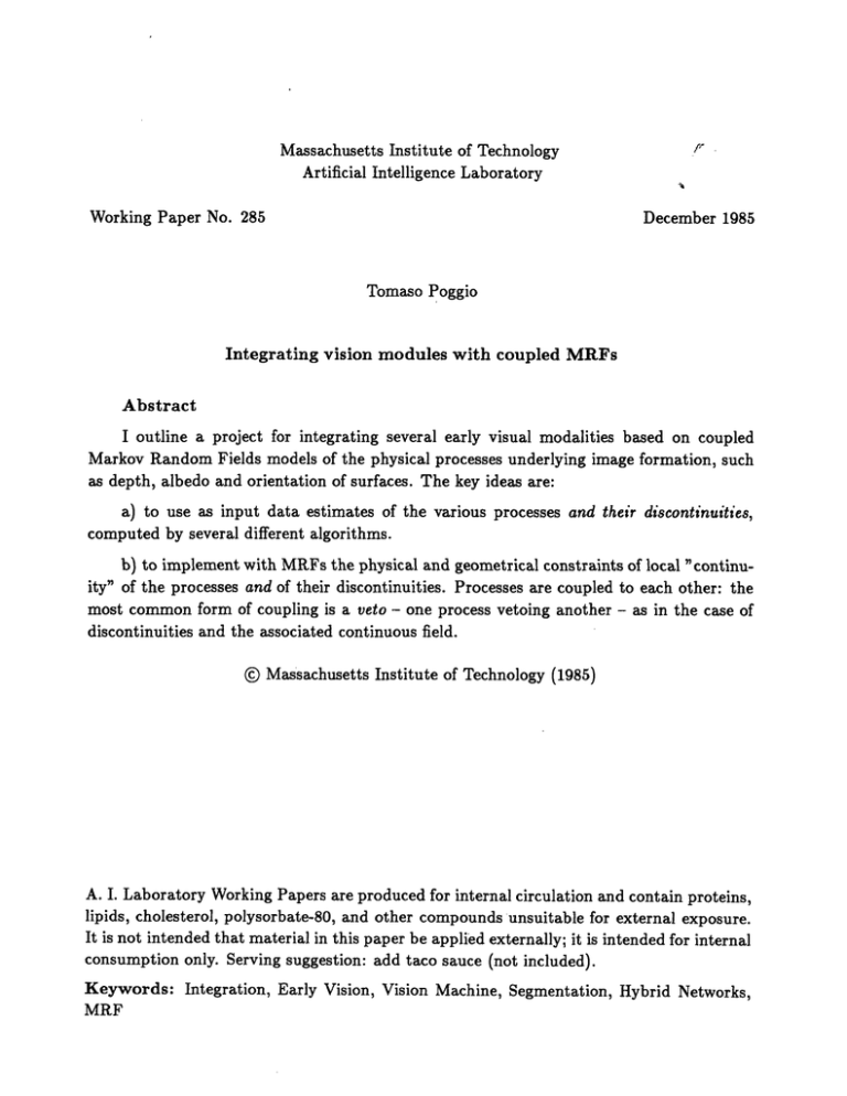
Massachusetts Institute of Technology
Artificial Intelligence Laboratory
Working Paper No. 285
December 1985
Tomaso Poggio
Integrating vision modules with coupled MRFs
Abstract
I outline a project for integrating several early visual modalities based on coupled
Markov Random Fields models of the physical processes underlying image formation, such
as depth, albedo and orientation of surfaces. The key ideas are:
a) to use as input data estimates of the various processes and their discontinuities,
computed by several different algorithms.
b) to implement with MRFs the physical and geometrical constraints of local "continuity" of the processes and of their discontinuities. Processes are coupled to each other: the
most common form of coupling is a veto - one process vetoing another - as in the case of
discontinuities and the associated continuous field.
© Massachusetts Institute of Technology (1985)
A. I. Laboratory Working Papers are produced for internal circulation and contain proteins,
lipids, cholesterol, polysorbate-80, and other compounds unsuitable for external exposure.
It is not intended that material in this paper be applied externally; it is intended for internal
consumption only. Serving suggestion: add taco sauce (not included).
Keywords: Integration, Early Vision, Vision Machine, Segmentation, Hybrid Networks,
MRF
Summary
Coupled Markov Random Fields provide a powerful method for integrating different
visual modules and for computing the equivalent of "intrinsic images" or a 21D sketch.
This paper outlines the math and the underlying ideas of this project. An implementation
is planned.
1) The key idea is that each visual modality (stereo, motion, texture, brightness and
color, etc.) provides measurements to two (or more) MRFs: one is continuous (or a discrete
approximation of a continuous field), the other is binary and corresponds to the discontinuities (that are critically important for segmentation in the VM project).
Typically, at least two different algorithms per modality attempt to measure "continuous" values and discontinuities, respectively. For instance, a motion algorithm attempts to
match features; a different "motion" algorithm attempts to find discontinuities in the motion
field. In the same way, there may be an unconventional stereo algorithm for finding uncorrelated regions, that correspond to occlusions. Thus several processes and combinations of
processes input data in the observable lattices.
2) The various MRFS mirror the different physical events that underly image formation:
surface, surface discontinuities, spectral albedo, albedo discontinuities, shadows, surface
normal, etc.
3) The local potentials underlying the a priori probability distribution of the MRFs
represent the constraints on the physical processes (smoothness, positivity, bounds etc.);
the coupling between MRFs represents the compatibility constraints between processes.
4) There are line processes (for discontinuities) and other types of binary veto processes.
5) The observable discontinuities provide a fast and coarse solution to the segmentation
problem. Using the MRFs for estimating the fields give an increasingly more precise solution,
simultaneously filling in the "continuous" regions that are only sparsely observable. The
solution at each iteration is available to later processes.
6) A parallel architecture for finding optimal estimators based on this model is a multilayered, coupled, hybrid network with local planar interactions and sparsely coupled in depth.
The Connection Machine is a good architecture for a first-order, fast implementation.
This scheme may provide a metaphor for the control structure underlying early vision.
It is possible, though - I believe - unlikely, that it will have a role in the VM project
as an alternative control metaphor to, say, the blackboard. I will also discuss it from the
point of view of evolutionary computation: is it possible to add layers (and their interactions)
successively without reconfiguring the whole network? This leads to another broad question:
how can the local potentials and the coupling interactions being improved by experience?
(A similar scheme may be interesting for speech understanding).
1.
Fusing modules makes vision systems possible
A reliable and robust vision system must exploit the integration of several different vision
algorithms and modalities. Not only contours but also stereo and motion and shading and
colour give information about depth, for instance. In addition, it is not unlikely that several
stereo algorithms are used. Whereas individual algorithms have to solve underconstrained
problems the combination of several modules may overconstrain.
A scheme that could
integrate this redundant information seem the only serious possibility today for developing
a vision system working on real images.
Caution Note: As Shimon says even small children are very good at recognizing monocular, monochromatic, still line drawings.
2.
The central role of discontinuities and their early detection
I believe that the main first step towards recognition is to segment the image in regions
that are likely to correspond to different objects. I believe that this segmentation pseudosegmentation -
has to be done very early on.
or
As a consequence, the detection
of discontinuities in the physical properties of surfaces has a critical role.
There must
be several different computations attempting to estimate the presence and the location of
discontinuities.
In some cases, discontinuities can be detected relatively easily. Several types of motion
discontinuities can be measured quite efficiently with simple operations on the time dependent intensity array, especially if the interframe interval is very small (see the example of the
fly's visual system). Albedo discontinuities may also be often detectable in terms of simple
operations. What about stereo? So far, all stereo algorithms not only do not directly detect
discontinuities in depth but perform badly precisely at occlusions. This state of affairs suggest the new idea that there may be a whole class of unexplored "stereo" algorithms with
the goal of detecting some of the occluded, rivalrous regions. There is some faint evidence
from psychophysics and physiology for this new role of "local" rivalry in depth perception
(more is up to Heinrich).
Notice that the goal of these early operations is a fast, rough detection of discontinuities
in order to guide other processes that will help the refinement of this initial estimate.
This point of view, if taken seriously, represents an almost complete turnaround of the
"traditional" approach (see Grimson, Terzopoulos etc.)
3.
Image Formation: the role of the physical processes
The fraction of light reflected from an object for each wavelength A depends on the light
source I(A), on the albedo p(x, A) and on the 3-D structure of the object. This last components can usually be described as a function of the directions of the viewer k, source s and
surface orientation n. Let i, e, g be the angles between n and s, n and k, and k and s. This
is expressed by
S(x, A) = p(x, A)E(x, A)
(1)
where S(x, A) is the image, E(x, A) = I(A)R(k, s, n, A) is also called effective irradiance
(see Hurlbert, 2001) and corresponds to the image produced by exactly the same 3-D scene
painted white. If the effective irradiance of a scene can be found, one can then think of the
albedo as a 2-D quantity: 3-D effects are all taken care of in E (and we are back to a flat
Mondrian-like world!). R is the reflectance function of the object.
The data measured by the sensors are:
SV(x)
=
a(A)p(x, A)E(A, [f])dA,
where v labels the spectral type of sensors (v
=
(2)
1, ...3 for R-G-B), a"(A) is the
spectral sensitivity of the vth-type sensor (or filter) and SV(x) its output. p(A,
•)
is the
surface albedo, E(A, f) is the effective irradiancethat takes into account 3-D shading effects
and possibly shadows and f is the surface z = f(x, y).
E is a functional of f (it usually
depends on the surface normal (through R), see Appendix).
Equation (2) shows that p and E cannot be determined from S and a uniquely without
additional constraints. In any case, there is clearly a factor - the relative scaling of E and
p - that cannot be determined unless the illuminant is observed directly.
4.
Some constraints on the physical processes can be captured
by MRF models
4.1.
The physical processes
Equation (1-2) show that some of the processes underlying image formation (under oversimplified assumptions) are
1) the surface depth z = f(x, y)
2) the albedo p(x, y, A)
3) the "effective irradiance" that usually depends on the surface normal and on the
illuminations
4) the surface normal n or equivalently the gradient space p, q
5) the illumination I(x, y, A) (this may be a dual process corresponding to two light
sources, a diffuse one and a point-like light source)
6) Other "minor" processes such as specularities or visible light sources that may locally
"veto" or "switch off" some of the previous processes.
Physical constraints apply to each of these processes independently. In addition, there
are constraints between these processes (for instance between z and n). Equation 1-2 show
how the image data constrain the way the processes combine. Notice that consideration of
time dependence will introduce additional powerful constraints such as rigidity. In the following I will neglect this important extension since because of its computational complexity
will not be taken into account in the first implementations.
The constraints on z, n, p are local conditions (such as smoothness, necessary mainly
because of its regularizing role in the face of omnipresent noise) valid everywhere but at
discontinuities. The rationale for this is discussed elsewhere (see for instance Marr and
also Poggio et al., 1985). Discontinuities are -
as we discussed -
critically important and
detected very early.
The machinery of coupled MRFs provides an ideal tool to impose the local constraints
of smoothness (plus others, such as positivity, values within certain bounds, etc.) allowing
at the same time an explicit role for discontinuities through the line process of Geeman
and Geeman (and similar processes such as occlusions, etc. see Poggio and staff, 1985 and
Marroquin et al., 1985). Here the new potentially powerful idea here is to have observable
discontinuity processes measured by specialized algorithms in different visual modalities.
Caution Note There are image properties however that do not seem easily captured
by MRF models. This is the case for instance of shadows and their dependence on the
illumination geometry and the surface values z = f(x, y). Intuitively, geometric constraints
of this type seem more "global" than what a MRF model can usefully represent. It is an
interesting question how to incorporate this in our present scheme.
4.2.
The constraints on the physical processes
We list here some of the constraints that can be exploited for each of the main processes
(including the associated discontinuity process):
a) Depth is smooth except at rare depth discontinuity lines that obey obvious geometric
constraints of continuity.
b) Typical illuminants and typical albedos have a finite (and small) number of degrees
of freedom. In other words, they can be described as linear combinations of a fixed set of
basis functions (notice that in different situations - such as different lighting conditions different bases may be required and that the illuminant basis is different, in general, from
the albedo basis). This assumption - called the spectral regularizationassumption has been
stated by several authors (see Hurlbert, 2001; for a recent review see Maloney, 1985).
c) Typically, E(x), the "effective irradiance", changes with x more slowly than R(x, A)
(apart from cases when surface changes abruptly or sharp shadows are present);
d) p(x, A) is either constant or changes sharply (at material edges). In many scenes, it
may be possible to assume that the average surface reflectance in each wavelength band is
'grey'.
e) Usually, the effective irradiance has the same dependence on x at each A:
E(x, A) = I(A)E(x)
(3)
This is equivalent to the assumption that R(x, A) in E(x, A) = I(A)R(x, A) (see equation
(1)) is, to a sufficient approximation, independent of A.
This is the single source assumption of Hurlbert and Poggio (see Hurlbert, 2001 and
Poggio et al., 1985)
f) The surface normal changes smoothly except at rare discontinuity lines
g) The illumination is smooth everywhere apart from rare shadow boundaries where it
changes discontinuously
h) For the depth, albedo, effective irradiance and illumination, it is possible to assume
certain upper and lower bounds for their admissible (or likely) values.
i) Discontinuities in each of these processes are typically continuous boundaries, locally
connected and non-intersecting.
Assumption b) allows one to rewrite Equation 2 as
S (x) = TC, eW(x)p, (x)
(4)
where the tensor T is defined as
S=1
av(A)pi(A)q i (A)dA
(5)
where v = 1, ...3 and i,j = 1, ...N, the p's and the q's are the basis functions for the
illuminant and for the albedo, respectively, and summation over repeated indices is tacitly
assumed.
Assumptions c) and d) mean that ei(x) will change slowly (apart from surface discontinuities) and pi(x) will be either constant or change sharply.
Assumption e) means that ei(x) = e'e(x). Thus the ratio between the intensity SV(x)
measured in one spectral channel and the intensity measured in another should change in
a noiseless situation only at albedo boundaries (where the albedo changes), and should be
invariant for changes in the effective irradiance.
5. Processes that deliver "continuous" data and processes that
measure discontinuities
There are several different algorithms to compute discontinuities in each of the physical
processes. We list here some of them. More will have to be considered in future work.
Depth discontinuities
a) One of the standard stereo algorithms may provide an estimate of location of possible
discontinuities by detecting regions of many weak matches, a situation typical for occlusions.
A possible stereo algorithm may itself be based on a MRF formulation (Marroquin et al.,
1985); furthermore a stereo algorithm can be coupled with the system outlined here in such
a way that influences in turn the matching itself.
b) A specialized stereo-rivalry algorithm may estimate regions that are likely to be
occluded
c) Motion discontinuities are usually an indication of depth discontinuities (especially
in the case of self-motion)
Albedo discontinuities
From the image the quantity D(x) =
is computed.
)
(we assume here for simplicity v = 1, 2)
Then we define the observation of the albedo discontinuity (Hurlbert and
Poggio, 2010; see Poggio et al., 1985) pt(i) (where 1 denotes the line process) as pt(i) = 1 if
an edge is detected at i and pI(i) = 0 otherwise. The presence of an edge is measured by
one of the "standard" edge detectors operating on D(x). Another independent algorithm
that estimates directly the albedo and the reflectance and could also be used simultaneously
is Yuille's (1984; see also Maloney, 1985). Notice that useful information can be obtained
if some properties of the illuminant can be measured (for instance by direct observation of
the light source).
Effective irradiance discontinuities
To find the discontinuities in the scene irradiance (or effective irradiance) we find all
edges in brightness and intersect this set with the set of albedo edges already found. The
edges that are not common are likely to be discontinuities in the scene irradiance, due
to either shadows or surface discontinuities or surface orientation discontinuities.
precisely, we perform edge detection on the brightness b(i) = E SV(x)].
More
We mark the
locations where an edge is by setting dbL = 1 and otherwise dbj = 0. We then compute an
estimate of the discontinuities in the effective irradiance as el(i) = dbl(i)(1 - Pt(i)), which
marks sharp changes of intensity likely to correspond to sharp changes in effective irradiance
but not changes in albedo (the threshold is set on the basis of noise estimates).
Texture discontinuities mark places that are not generic discontinuities in the effective
irradiance (they are not shadows and they are not sharp changes in the surface orientation).
Surface normal discontinuities and illumination discontinuities
They may be inferred exploiting additional information such as knowledge that the
reflectance function is lambertian and labeling of brightness edges as shadows (using for
instance measurements of texture on the two sides of an edge).
There is much to do for developing several algorithms that provides the measurements of
discontinuities in the different processes, exploiting different cues. It is especially important
to have independent estimates of the same type of discontinuities: the weight they have,
if two or more estimates coincide at a specific location, is large (see later), indicating very
strongly the presence of a discontinuity.
One possibility to be considered in a second stage is that these estimation processes
are themselves coupled with the lattices of the physical processes. In this way the estimate
of depth at time to in the 21D sketch will influence the operation of gathering depth data
at later times (changing parameters in the input algorithm or by coupling to a MRF based
stereo algorithm, see Poggio and Yuille, who are presently sweating about it).
6.
6.1.
A model of Early Vision
The basic physical processes
The basic local constraints on the "continuous" physical processes can be captured by assuming that they are MRF. In this case their a priori probability distributions are Gibbs
with basic potentials that I give here as a semi-serious illustration. I assume for simplicity
time independent imagery (and relegating therefore motion to a secondary position: this is
certainly not true for real-life, real-time vision) and 1-D notation.
1) The depth process is a MRF with a potential of the type
U (z) = U(z(i),z(j)) = (z(i) - z(j))2
=0
fori-jl
1
otherwise
(6)
Lower and upper bounds on the depth process can be introduced with a potential term
of the following flavor
Uboun d = 0
= LN
lb < z < ub
otherwise
(7)
where LN is a large number. Depth can also be assumed to be piecewise constant in
which case the potential equation (11) would be somewhat different.
2) Another (vector) MRF corresponds to the albedo p(x) with components in 2 or 3
spectral bands with values p(x) on the lattice. Assumption c) suggests a potential
Up(p) = U(p,,pi) = #((Pi - Pj) 2 )
= 0
forli - jl = 1
otherwise
where ((z) is a symmetric function that is 0 for z = 0, is large for small values of jzl,
and may go to 0 again for large values of |zl (a standard Ising model may actuallly suffice,
see Marroquin et al., 1985).
In this way slow changes of p are penalized, whereas either
constant values or sharp changes carry no cost.
Lower and upper bounds on the albedo process (they are surprisingly strict because of
the physics of surfaces) can be introduced with a potential term similar to equation (8).
3) The "effective irradiance" is defined as a (vector) MRF, corresponding to the illuminant components in 2 or 3 spectral bands with values e(x) on the lattice. We chose these to
satisfy Assumption 2. For instance (neglecting vector notation because of TEX problems)
Ue(e) = U(e, ej) = (e- - ej) 2
= 0
forli -
l = 1
otherwise
(9)
Again, lower and upper bounds can be imposed with a potential term similar to equation
(12).
4) The surface normal would also obey to a potential U, similar to the depth process.
5) The illumination I would have a potential Ui similar to U,.
6.2.
Discontinuity processes
In order to respect the previous assumptions that mostly impose smoothness everywhere
except at (rare) discontinuities we introduce for each of the physical processes f a binary
discontinuity process fi. This process has an associated potential reflecting the geometrical
properties of boundaries (mainly that they are piecewise smooth curves, that there cannot
be too many of them and that they do not intersect). I do not write explicitly these terms
here. Their form is similar to Geman and Geman's and Marroquin's. The corresponding
potentials are Uzz, Up,, Ue,, Us,, Ui,.
6.3.
Coupling the "continuous" MRF to their (observable) discontinuities
Each process f is coupled to its discontinuity by multiplying Uf with (1 - fL).
6.4.
Introducing "continuous" observations
We introduce the "continuous" data Z (depth) and S (color brightness) obtained as explained earlier by assuming that Z(x) and S (x) correspond to samples of signals affected by
additive gaussian noise. The corresponding potential terms in the a posteriori distribution
are of the type
Uz=-
(Z(i)
-
z(i)) 2
Us = 1-(-S((i) - T,e(i)p (i))2
(10)
(11)
20
In equation (11) we have coupled the effective irradiance to the albedo.
6.5.
Introducing discontinuous observations
The discontinuity processes are observable in our framework. Their observation model has
the typical potential
u(yf,t) = a•
(1 - 6(fi(i) - t(i)))
(12)
where 6 is the delta function, fd is the discontinuity process, and t is the observation.
In the case of an error rate c for a binary symmetric channel a is a = In
If more than one independent observation is available for the same discontinuity process (say two different algorithms estimate discontinuities in Z, providing the discontinuity
indeces tl and t2) then each will contribute a term as the previous equation plus a joint
term with a form of the type
U, (fl,tl,t2) = X
where X = In
6.6.
(1 - 6(fd(i) - tl(i)t2(i)))
(13)
•
Coupling the processes
The irradiance equation equation 1) allows us to couple some of the processes. We have
done this already for the effective irradiance and the albedo. If the reflectance is lambertian
then equation 6 shows how I and R are coupled to E: under the assumption of gaussian
additive noise (for instance) the corresponding potential term is of the form
12
6.7.
(E(i) - I(i)R(i))2
(14)
A very simple model
In the case of just three processes (depth, albedo, effective irradiance) and their discontinuities, the total potential corresponding to the a posteriori Gibbs distribution is then
Up(z,p,e, z, p,,e) =
Uz + Us + (1 - z 1 )U, + (1 - pt)UP + (1 - el)Ue+
+Uz 1 + Upi + Uge + U(z, t) +...
+Ubzound + ...
(15)
It is not too difficult to insert the additional terms corresponding to other processes
such as surface normal etc. and their coupling. For instance, the surface normal would be
coupled to the z process by a potential term of the form
2K2
6.8.
z
p) 2 + (z2y - q) 2
(16)
Estimation
As a performance criterion we will use a mixed criterion, where z, e and p should be as close
as possible to their true values and we should make as few errors as possible in the assertion
about the presence or absence of discontinuities.
Thus the optimal estimates are the posterior mean for z and e' and pV (or the thresholded posteriori mean if they are processes with discrete values) and the maximizer of the a
posteriori marginals for zz, pi, el, nl, it. We can compute these estimates by using Montecarlo methods of the type discussed by Marroquin (1985a,p. 132, 1985; see also Marroquin
et al., 1985), running at a constant temperature.
7.
7.1.
Conclusions
The real problem and the implementation
The main problems of this scheme are
a) how to set the values of the coupling constants (they depend on noise estimate
and on the "natural" temperature of the individual processes).
Note that one expects
possible discontinuous behaviour of the system as a function of the parameters because of
its nonlinearity and cooperativity (think of the Ising model).
b) computational complexity, possibly implying less-than-real-time performance even
on powerful parallel computers.
c) intrinsic locality of the Markov assumption that makes very difficult to consider more
global properties, such as shadows.
d) stationarity assumption underlying the probabilistic formulation.
One way to explore these issues is to implement the scheme sketched in this paper (on
the 3600 or even the CM). This is what I plan to do.
7.2.
Extensions and alternatives
A possible alternative application of MRFs that may be of special interest for the Vision
Machine project, is to use MRFs on graphs instead than lattices (see Kindermann and Spell,
1980). In this way, it may be possible to integrate symbolic descriptions that are not pixel
based as in the scheme of this paper.
An important extension of the scheme outlined here is to time-dependent scenes. First,
however, the sheme should show some promises on still imagery. Many other obvious extensions were not mentioned. Multiple scales must be taken into consideration; higher level
control is needed; a small expert system may adjust the parameters of the coupled MRFs,
depending on statistical measurements on the fields and a small set of heuristics.
7.3.
An evolutionary view of computation
The scheme outlined here is a possible control structure for a Vision Machine (though I do
not believe it is the "right" approach). An ideal control structure would have the property
that new modules can be added at will without having to change the control code. This
property is important in a project like the CVM that involves several people and attempts
to develop with time an increasingly sophisticated system. It must be essential to evolution
which does not have ever the possibility to "rewrite" code from scratch when it becomes
too unwieldy. Does the MRF model have this property? It seems possible that it may.
When a new term is added to the potential it will not affect much the other lattices as long
as the coupling constant is small. In a sense, it will be a kind of "neutral" mutation. For
this reason it may be a good strategy to add new potential terms (corresponding to new
processes or interactions among them) that at first are quadratic and have a small coupling
coefficient. The constant may increase and their shape become less convex under selection
pressure.
7.4.
Learning
A clearly important problem is to develop (possibly very slow) schemes to estimate the
optimal parameters of the potential from examples of succesful computations. This may be
the only practical way of setting the parameters of this model: learning from experience. Is
this possible?
As a side remark, that may or may not be relevant, I believe that learning can be
succesfull only if the system has almost learned, in the following sense. One can think of
learning as a two stage process: in the first stage, one sets up the representations, in the
second stage, operators are learned. In a simple associative learning - for instance, learning
to associate names to faces - learning requires setting the features to be used and then
associating them. It can be proved that the general nonlinear "black-box" that has to be
synthetized during learning is equivalent to two "boxes" corresponding to these two steps
(Poggio, 1983). The first one can be regarded as a nonlinear coding step, whereas the second
one is a linear operator. It is clearly tempting to think that a slow, almost exhaustive search,
such as evolution, takes care of the first step whereas much faster "learning" synthetize the
second "box". In a similar way, learning in our MRF model should probably be restricted
to parameter estimation of an already existing model.
7.5.
Connection with previous work
Once this blurb was conceived and almost completely written, I discovered something I
should have known, that is that Barrow and Tennenbaum (1978) had sketched ideas with a
lot in common with the present scheme. In particular, they stated explicitely the photometric constraints, the use of intrinsic images corresponding to the physical processes undelying
image formation, their local constraints, the role of discontinuities. They do not have the
machinery of MRF and the equations to develop a succesfull implementation (they did not).
They gloss over the "details" of how their model can be made to work. They do not have
clear enough the role and the description of the processes that must measure properties of
the fields and of their discontinuities. This, I believe, is a major point, which requires much
research. This research, by the way, will be valid independently of whether the MRF-based
fusion scheme proposed here is correct. It represents therefore the major justification for
working on this project.
7.6.
Work to be done
I do not spell in detail the obvious and less obvious questions to be answered. There are
several in the field of MRF theory, in estimation, in parallel implementations, in the development of efficient and simple algorithms for providing the initial measurements and
especially in psychophysics, concerning the role of discontinuities, their early and independent detection and the fusion of information about different physical processes.
Acknowledgments
Thanks to Jim Little who not only signed but also read this draft and made several
corrections and improvements.
Appendix: Parenthesison lambertian surfaces
Many surfaces can be modelled as combinations of Lambertian and specular surfaces.
Lambertian surfaces look equally bright from all directions. Their reflectance function RL
can be written as
RL = s -n = cos(i)
(Al)
In many cases R depends only on the normal of the surface. An arbitrary point on a
surface z = f(x, y) is given by
r = (x, y, f(x, y)).
(A2)
The surface normal is
1
n =(-f
1
(1 + fX + fy2) /21),
-l1)5
(A3)
(A3)
where fx and fy are the partial derivatives of f with respect to x and y. They are
usually denoted by p and q respectively. The coordinate frame based on (p, q) is also called
Gradient Space.
In this space a planar patch ax + by + c = z corresponds to a point
p = a, q = b. Using this notation the image irradiance equation becomes
E(x, y, A) = I(A)R(p, q).
(A4)
READING LIST
Brooks,M.J. and Horn, Berthold K.P. "Shape and Source from Shading", A.I. Memo
720 (1985)
Buchsbaum, G. "A spatial processor model for object color perception," J. Franklin
Inst., 310, 1980.
Canny, John F. "Finding edges and lines," Massachusetts Institute of Technology Technical Report 720, 1983.
Geman, Stuart, and Don Geman. "Stochastic relaxation, Gibbs distributions, and the
Bayesian restoration of images," IEEE Trans. Pattern Analysis and Machine Intelligence,
6, 1984.
Grimson, W.E.L. From Images to surfaces, Massachusetts Institute of Technology
Press, Cambridge, Mass., 1981.
Hillis, D. "The Connection Machine," Massachusetts Institute of Technology Department of Electrical Engineering and Computer Science Ph.D. Thesis, 1985.
Horn, Berthold K.P. Robot Vision, MIT Press and McGraw-Hill (1985).
Horn, B.K.P., "Obtaining shape from shading information", in: The Psychology of
Computer Vision, P.H. Winston, ed., McGraw-Hill Publ., New York, 115-155, 1975.
Horn, B.K.P., "Understanding image intensities", Artificial Intelligence, 8, 201-231,
1977.
Hurlbert, Anya. "Color computation in the visual system," Massachusetts Institute of
Technology Artificial Intelligence Laboratory Memo 814, 2001, in press.
Kirkpatrick, S., Gelatt, C.D., Jr., and Vecchi, M.P. "Optimization by simulated annealing," Science, 220, 1983.
Land, Edwin H. "Recent advances in retinex theory and some implications for cortical
computations: colour vision and the natural image," Proceedings of the National Academy
of Sciences, 80, 1983.
Maloney, Laurence T. "Computational approaches to color constancy" Stanford University Tech. Report 1985-01, 1985.
Marr, David. "Early processing of visual information," Phil. Trans. R. Soc. London
B275, 1976.
Marroquin, J. 1984 "Surface reconstruction preserving discontinuities," Massachusetts
Institute of Technology Artificial Intelligence Laboratory Memo 792, 1984.
Marroquin, J. "Optimal bayesian estimators for image segmentation and surface reconstruction," Massachusetts Institute of Technology Artificial Intelligence Laboratory Memo
839, 1985.
Marroquin, J. "Probabilistic solution of inverse problems," Ph.D. Thesis, Massachusetts
Institute of Technology , 1985.
Marroquin, J., Mitter, S. and Poggio, T. "Probabilistic solution of Ill-posed problems in
Computational Vision" Proceedings Image Understanding Workshop, Baumann ed., SAIC,
1985.
Metropolis, N., A. Rosenbluth, M. Rosenbluth, A. Teller, and E. Teller. "Equation of
State Calculations by Fast Computing Machines," J. Phys. Chem. 21, 1953.
Poggio, T. and the staff "MIT Progress in Understanding Images", Proceedings Image
Understanding Workshop, Baumann ed., SAIC, 1985.
Poggio, Tomaso, Vincent Torre, and Christof Koch. "Computational vision and regularization theory," Nature 317, 1985.
Rubin, John, and Whitman Richards.
"Colour Vision: Representing Material Cat-
egories," Massachusetts Institute of Technology Artificial Intelligence
764, 1984.
Laboratory Memo
21
Terzopoulos, Demetri. "Regularization of inverse visual problems involving discontinuities," IEEE Trans. Pattern Analysis and Machine Intelligence, 1986, in press.
Yuille, Alan L. "A method for computing spectral reflectance," Massachusetts Institute
of Technology Artificial Intelligence Laboratory Memo 752, 1984.
I
I
IN
N
N
N
N
N
~
N
N
N
-.
'-4
-o
0
J
Ph
a4
m
m
o
P
r
-tl
rm
-l
FROM EARLY PROCESSING
FROMEARLY PROCESSING