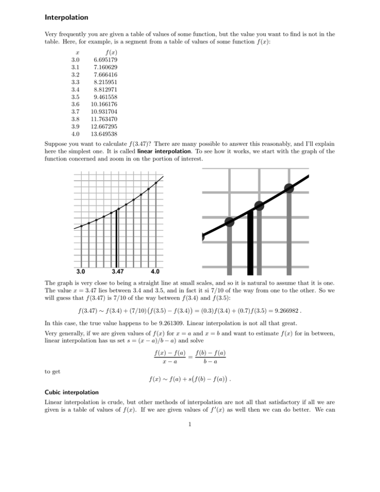
Interpolation
Very frequently you are given a table of values of some function, but the value you want to find is not in the
table. Here, for example, is a segment from a table of values of some function f (x):
x
3.0
3.1
3.2
3.3
3.4
3.5
3.6
3.7
3.8
3.9
4.0
f (x)
6.695179
7.160629
7.666416
8.215951
8.812971
9.461558
10.166176
10.931704
11.763470
12.667295
13.649538
Suppose you want to calculate f (3.47)? There are many possible to answer this reasonably, and I’ll explain
here the simplest one. It is called linear interpolation. To see how it works, we start with the graph of the
function concerned and zoom in on the portion of interest.
3.0
3.47
4.0
The graph is very close to being a straight line at small scales, and so it is natural to assume that it is one.
The value x = 3.47 lies between 3.4 and 3.5, and in fact it si 7/10 of the way from one to the other. So we
will guess that f (3.47) is 7/10 of the way between f (3.4) and f (3.5):
f (3.47) ∼ f (3.4) + (7/10) f (3.5) − f (3.4) = (0.3)f (3.4) + (0.7)f (3.5) = 9.266982 .
In this case, the true value happens to be 9.261309. Linear interpolation is not all that great.
Very generally, if we are given values of f (x) for x = a and x = b and want to estimate f (x) for in between,
linear interpolation has us set s = (x − a)/b − a) and solve
f (b) − f (a)
f (x) − f (a)
=
x−a
b−a
to get
f (x) ∼ f (a) + s f (b) − f (a) .
Cubic interpolation
Linear interpolation is crude, but other methods of interpolation are not all that satisfactory if all we are
given is a table of values of f (x). If we are given values of f 0 (x) as well then we can do better. We can
1
approximate the function between x = a and x = b by the unique cubic polynomial P (x) which has the same
function values and the same derivatives at both a and b. I won’t give details, but this leads to
∆x = b − a
x−a
s=
b−a
f (x) ∼ f (a)(1 − s)3 + 3s(1 − s)2 f (a) + (1/3)f 0 (a)∆x
+ 3s2 (1 − s) f (b) − (1/3)f 0 (b)∆x + f (b)s3
For the same function as before we have this extended table:
x
3.0
3.1
3.2
3.3
3.4
3.5
3.6
3.7
3.8
3.9
4.0
f (x)
6.695179
7.160629
7.666416
8.215951
8.812971
9.461558
10.166176
10.931704
11.763470
12.667295
13.649538
f 0 (x)
4.463453
4.850748
5.270661
5.726270
6.220920
6.758256
7.342238
7.977189
8.667821
9.419270
10.237153
Cubic interpolation gives the estimate 9.261308, which is off only in the last digit.
2