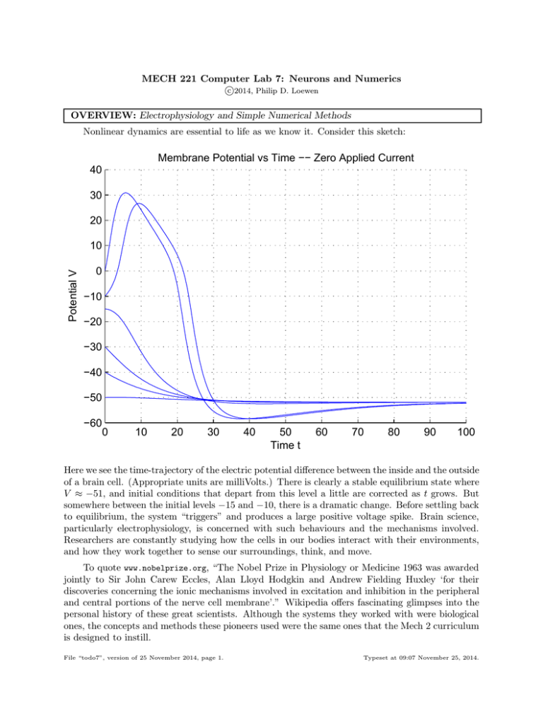
MECH 221 Computer Lab 7: Neurons and Numerics
c 2014, Philip D. Loewen
OVERVIEW: Electrophysiology and Simple Numerical Methods
Nonlinear dynamics are essential to life as we know it. Consider this sketch:
Membrane Potential vs Time −− Zero Applied Current
40
30
20
Potential V
10
0
−10
−20
−30
−40
−50
−60
0
10
20
30
40
50
Time t
60
70
80
90
100
Here we see the time-trajectory of the electric potential difference between the inside and the outside
of a brain cell. (Appropriate units are milliVolts.) There is clearly a stable equilibrium state where
V ≈ −51, and initial conditions that depart from this level a little are corrected as t grows. But
somewhere between the initial levels −15 and −10, there is a dramatic change. Before settling back
to equilibrium, the system “triggers” and produces a large positive voltage spike. Brain science,
particularly electrophysiology, is concerned with such behaviours and the mechanisms involved.
Researchers are constantly studying how the cells in our bodies interact with their environments,
and how they work together to sense our surroundings, think, and move.
To quote www.nobelprize.org, “The Nobel Prize in Physiology or Medicine 1963 was awarded
jointly to Sir John Carew Eccles, Alan Lloyd Hodgkin and Andrew Fielding Huxley ‘for their
discoveries concerning the ionic mechanisms involved in excitation and inhibition in the peripheral
and central portions of the nerve cell membrane’.” Wikipedia offers fascinating glimpses into the
personal history of these great scientists. Although the systems they worked with were biological
ones, the concepts and methods these pioneers used were the same ones that the Mech 2 curriculum
is designed to instill.
File “todo7”, version of 25 November 2014, page 1.
Typeset at 09:07 November 25, 2014.
2
MECH 221 Computer Lab 7: Neurons and Numerics
The Hodgkin-Huxley Model is a system of 4 ordinary differential equations in 4 unknowns
that is still the subject of intense research for modelling the activity of neurons and muscles in
all kinds of organisms. For the sake of simplicity, we consider here a simplified 2-variable system
known as the Morris Lecar Model. The state vector is (V, N ), where V is the voltage drop
across a cell membrane and N is a dimensionless “recovery variable” related to chemical dynamics
and probability. The differential equations are
C
dV
= Iapp − gCa Mss (V )(V − VCa ) − gK N (V − VK ) − gL (V − VL ),
dt
Nss (V ) − N
dN
=
.
dt
τ (V )
(1)
(2)
They involve constant conductances gCa , gK , gL and reference potentials VCa , VK , VL associated with
Calcium ions (Ca2+ ), Potassium ions (K+ ), and Leakage (suspected to be Chloride ions, Cl− ). To
simplify the presentation above, three auxiliary functions have been used:
V − V1
1
,
(3)
Mss (V ) = 2 1 + tanh
V2
V − V3
1
,
(4)
Nss (V ) = 2 1 + tanh
V4
1
.
τ (V ) =
(5)
−V3
φ cosh V2V
4
These involve constant parameters V1 , V2 , V3 , V4 , φ. The formulation quoted here comes from
Wikipedia1 ; see also the Scholarpedia page2 maintained by Lecar himself.
Students experienced in circuits will recognize the beginning of Equation (1), C dV
dt = Iapp , as
the law relating current and capacitance. The remaining terms in (1) are produced by applying the
Kirchhoff Current Law to a node where the applied current feeds not only a capacitor (our model
for the cell membrane), but also three resistors wired in parallel across the capacitor. The simplest
term, gL (V − VL ), describes the leakage current using Ohm’s Law. (The conductance, g, is simply
the reciprocal of the resistance.) The other terms are complicated because electric current through
a membrane measures motion of big massive ions through protein-controlled gates, rather than tiny
lightweight electrons along a wire. In cells, different channels are tuned to different ions, and their
conductance depends on relative ion concentrations and electric potential in ways too complicated
to summarize here.
In this lab we will combine standard ODE methods and computer solutions to solve initialvalue problems for (V (t), N (t)) based on system (1)–(5). We will use the parameter values selected
by Mike Martin for his online Morris-Lecar simulator,
http://math.jccc.edu:8180/webMathematica/JSP/mmartin/morlecar.jsp
Running the simulator3 is a convenient way to verify our calculations in the lab.
Numerical Methods. The system (1)–(5) is too hard to solve by hand. But we can use the
“velocity field” idea to generate approximate solutions. And if we step back from our particular
1
2
https://en.wikipedia.org/wiki/Morris-Lecar_model
http://www.scholarpedia.org/article/Morris-Lecar_model
3
Link checked on 2014-11-23 by Philip D. Loewen.
File “todo7”, version of 25 November 2014, page 2.
Typeset at 09:07 November 25, 2014.
MECH 221 Computer Lab 7: Neurons and Numerics
3
unknown vector y(t) = (V (t), N (t)) to a general time-varying y = y(t) in Rn , we will have a tool
that can be used for all kind of ODE systems.
Consider an initial-value problem for a general time-varying vector y(t) in Rn , in the form of
a system of first-order ODE’s:
ẏ(t) = G(t, y(t)), t ≥ t0 ;
y(t0 ) = y0 .
(1.1)
Given a starting time t0 and corresponding initial state y0 , we seek to identify the function y = y(t)
whose vector velocity at every instant exactly matches the value prescribed by the given function
G.
Discretization. The basic idea starts by specifying a list of times
t0 < t1 < . . . < tN
for which we would like to know the values of the exact solution. Let’s use the notation yk for our
computed approximation to the exact value y(tk ). Since y(t0 ) is given, we know y0 . For all k ≥ 1,
the exact value y(tk ) may never be known; our goal is somehow to generate a good approximation.
Euler’s Method. Pick a subscript k for which yk−1 is known. To calculate yk , . . .
1. Find the (vector) velocity associated with the known previous point, namely,
E
vk−1
= G(tk−1 , yk−1 ),
2. Use that velocity with previous location and time duration to complete the job, defining
E
yk = ykE = yk−1 + (tk − tk−1 )vk−1
.
Since y0 is known, we can use these steps with k = 1. Then y1 will be defined at the end of step
2, so we can loop back and repeat the process.
Heun’s Method. The so-called “Improved Euler” method, due to Heun, modifies the velocity
calculation suggested above.
1. Calculate a (vector) velocity by averaging the value at the previous point (tk−1 , yk−1 )
with the value associated with the point that Euler’s method would move to next:
H
vk−1
=
G(tk−1 , yk−1 ) + G(tk , ykE )
,
2
2. Use that velocity to move forward as before, defining
H
yk = ykH = yk−1 + (tk − tk−1 )vk−1
.
Heun’s approximations turn out to be far better than Euler’s, as we will see in the lab.
File “todo7”, version of 25 November 2014, page 3.
Typeset at 09:07 November 25, 2014.
4
MECH 221 Computer Lab 7: Neurons and Numerics
LAB ACTIVITIES, PART ONE: Handcrafted ODE Solvers
1. Download testspring.m from Connect and run it. You should get two plots showing solutions
computed by ode45 for the familiar initial-value problem
ẍ(t) + x(t) = 0,
x(0) = 1, ẋ(0) = 1.
The exact solution is known: x(t) = cos(t) + sin(t), with ẋ(t) = cos(t) − sin(t) and energy
E(t) = 21 ẋ(t)2 + 12 x(t)2 = 1.
Each plot uses a different number of equal subintervals for the same time interval, [0, 8π]. The
version of testspring on connect uses an unreasonably small number of subintervals. Edit
testspring to use more subintervals, and to produce 3 plots instead of 2. (Suggested counts:
256, 512, 1024, etc.) Then re-run it and compare the results to your expectations.
2. Notice that testspring.m is structured to apply up to three different solvers for the given IVP.
A few minor edits will make the script use a solver named ode01 in addition to ode45. Activate
this feature, and then write the corresponding function ode01. As the code in testspring
suggests, ode01 should consume exactly the same inputs as ode45, and return values with just
the same interpretations. Internally, however, your function ode01 should use Euler’s method
to solve whatever IVP it is given.
Like ode45, your function ode01 must deal with its input function G in general, so that it can
be used on any given differential equation with a vector unknown y = y(t) of any dimension.
Use testspring to confirm that your implementation of Euler’s method is working.
Preview : Euler’s method is famously inaccurate. Even a perfect implementation will produce
results that start out similar to the correct ones, but drift away as time advances. Accuracy
should improve as the number of subintervals in [0, 8π] is increased, but it will never be great.
3. Write a second solver, named ode12, using Heun’s method (also known as the “Improved Euler”
method). Make the minor edits to the script testspring so that it applies each method—Euler,
Heun, and ode45—to your three chosen subdivisions of the basic interval.
4. Let xE (N ) denote the value of x(8π) predicted by Euler’s method using N subintervals. (The
initial conditions never change.) Estimate the constant C = CE and the integer exponent
γ = γE for which
γ
1
for N ≫ 1.
xE (N ) ≈ 1 + C
N
Suggestion: Calculate xE (N ) for various N (e.g., N = 256, 512, 1024, 2048, 4096) using your
script. Then plot ln(xE (N ) − 1) versus ln(1/N ) using any method you like (Matlab, Excel, or
calculator), fit a straight line, and analyze the slope and intercept to find C and γ.
5. Let xH (N ) be the value of x(8π) predicted when Heun’s method is applied with N subintervals.
Find the constant C = CH and exponent γH such that
γ
1
for N ≫ 1.
xH (N ) ≈ 1 + C
N
6. Prepare to hand in your function ode01, your computed values of xE (N ) for various N , and
your estimates for C and γ in the Euler-method case, with some description of your methods.
Do the same for ode12 and the Heun-method counterparts of all these elements.
File “todo7”, version of 25 November 2014, page 4.
Typeset at 09:07 November 25, 2014.
MECH 221 Computer Lab 7: Neurons and Numerics
5
LAB ACTIVITIES, PART TWO: Morris-Lecar Studies with Iapp = 0
1. Get the file MorrisLecar0.m from Connect and look through it carefully. There you will find
all the parameter values needed to be completely specific about the Morris-Lecar model in
equations (1)–(5) above, along with explicit definitions of the helper functions in lines (3)–(5).
It may be helpful later to copy-paste elements of this file into other places.
Note: The file/function name includes the character 0 because it implements only the special
case of equation (1) in which Iapp = 0. This special case applies to all activities on this page.
2. Assuming Iapp = 0, set up a plot of the phase plane for the Morris-Lecar Model. Work in the
box where V runs along the horizontal axis, N runs along the vertical axis, and the intervals
of interest are
−70 ≤ V ≤ 50,
−0.2 ≤ N ≤ 1.
You will probably want to write a script to do this, perhaps modifying a script you have used
in the past instead of starting from a blank screen. The desired plot will show
⊔ The nullclines—that is, the (V, N ) points in the box where one of dV /dt = 0 or dN/dt = 0.
⊓
These are pretty easy to deduce from equations (1)–(2), but since the system is nonlinear
its nullclines are curves, not straight lines.
⊔ A reasonable sampling of velocity vectors, suitably scaled and/or truncated as described
⊓
in the paragraph headed “Velocity Field” on page 2 of the writeup for Computer Lab 5.
Tip: The arrow-drawing function vec2d used in Computer Labs 5 and 6 works badly here,
because the scales are so different on the two axes. So forget about drawing fancy little
arrowheads: just plot the velocity vectors as blunt little segments using the plot command
instead of vec2d.
3. Continuing with Iapp = 0, use ode12 to solve the Morris-Lecar equations with a variety of
initial conditions, and thereby reproduce the plot shown on page 1 of this writeup. For each
trajectory on that plot, draw the corresponding path in the phase plane.
Details: Use the time interval 0 ≤ t ≤ 100, with some reasonable number of intermediate
nodes. Use N (0) = 0 in all cases, but choose the following values for V (0):
−50, −40, −30, −15, −10, 0.
4. Write a function named peakvalue that takes a single scalar input c and returns the scalar value
m defined as follows: m is the maximum value over 0 ≤ t ≤ 100 for the function V (t) produced
by running the Morris-Lecar model with initial conditions (V (0), N (0)) = (c, 0). (Continue
with Iapp = 0.) The sketch on page 1 suggests that peakvalue(c) is approximately equal to c
when c < −20, but then peakvalue(−10) is between 25 and 30, and peakvalue(0) is above 30.
Plot the graph of the function peakvalue for the interval −50 ≤ c ≤ 0.
5. Find, with 3-figure accuracy, the initial voltage c near −10 for which the peak value is 20.0.
Hint: This task is equivalent to solving for c in f (c) = 0, where f (c) = peakvalue(c)-20. We
have tools for this kind of task—notably the function findzero we built in Computer Lab 3.
You may apply that function, or use Matlab’s built-in fzero, or do something crude by hand.
6. Prepare to hand in your phase plane plot showing the elements listed in Item 2 and the
trajectories in Item 3. Also hand in your definition of the peakvalue function, the graph
requested in Item 4 and the mystery voltage calculated in Item 5 (with a brief explanation of
your method).
File “todo7”, version of 25 November 2014, page 5.
Typeset at 09:07 November 25, 2014.
6
MECH 221 Computer Lab 7: Neurons and Numerics
LAB ACTIVITIES, PART THREE (OPTIONAL): Bias Current and Steady Oscillations
Most students will be out of time by this point, so everything on this page is optional. But it’s also
easy and fascinating. Here we make minor changes to the work in Part Two to allow for a steady
applied current of Iapp = 100.
1. Consider the Morris-Lecar system with Iapp = 100. Plot the nullclines and velocity field, as in
Part Two.
Note that one of the nullclines moves to a new position when we change Iapp .
2. Continuing with Iapp = 100, solve the Morris-Lecar equations on the longer time interval
0 ≤ t ≤ 500. Use your own ode12 if you can, and fall back onn Matlab’s ode45 if you must.
Draw not only the phase plane trajectory, but also the graphs of V (t) and N (t). Use the initial
conditions V (0) = −20, N (0) = 0.
3. Continuing with Iapp = 100, explore the phase plane by adding trajectories with other initial
states on the vertical line in the phase plane where V = −20.
4. In Part Two above, we used Iapp = 0 and managed to trigger a single pulse for sufficiently
large initial voltages. Here, with Iapp = 100, we get a periodic pulse-train for most initial
voltages. It’s reasonable to expect the transition from one spike to infinitely many to occur
at some intermediate level of Iapp . Locate this transition level somehow: trial-and-error is one
possibility. Can you suggest something automated?
5. Since this activity is optional, there is no prescribed format for the final submission. Produce
whatever documentation you think is appropriate, and discuss it in person with the lab TA
and/or your instructor.
File “todo7”, version of 25 November 2014, page 6.
Typeset at 09:07 November 25, 2014.