EE353 Lecture 20: Introduction to Random Processes
1
EE353 Lecture 20: Intro To Random Processes
Chapter 9: 9.1: Definition of Random Processes
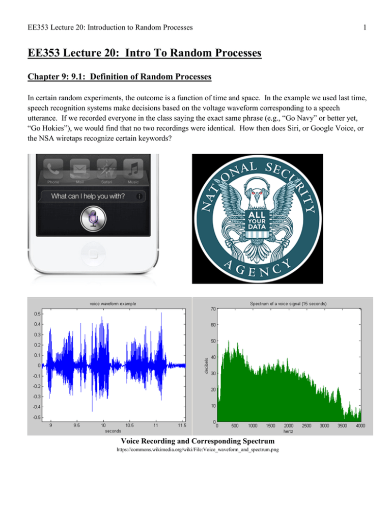
In certain random experiments, the outcome is a function of time and space. In the example we used last time,
speech recognition systems make decisions based on the voltage waveform corresponding to a speech
utterance. If we recorded everyone in the class saying the exact same phrase (e.g., “Go Navy” or better yet,
“Go Hokies”), we would find that no two recordings were identical. How then does Siri, or Google Voice, or
the NSA wiretaps recognize certain keywords?
Voice Recording and Corresponding Spectrum
https://commons.wikimedia.org/wiki/File:Voice_waveform_and_spectrum.png
EE353 Lecture 20: Introduction to Random Processes
2
Taking it one step further, what about those wonderful biometric
identification systems (such as the fingerprint scanner, hand geometry
scanner, iris recognition, or voice recognition over in the ECE
Biometrics Lab)? What if your phone is locked via your voice and if
you get a cold? Does that mean you can no longer access your phone?
What if your classified iPad is biometrically locked to your specific
EKG pattern (don’t laugh; Dr. Anderson was one time part of a panel
discussion on this very topic). What if you’re taking heavy fire or are
otherwise in a stressful situation, does that mean you can’t access the
SIPRNET?
Clearly something else must be going on here to support those
applications.
Biometrics are Cool
https://commons.wikimedia.org/wiki/File:Biometric.jpg
The functions in the above examples can be viewed as numerical quantities that evolve randomly as a
function of time or space. What we really have then is a family of random variables indexed by the time or
space variable. For the final part of the course, we will investigate these random processes.
Important Distinction
A sine-wave is a deterministic signal. Given the frequency, amplitude and initial phase offset, we can
predict/determine what its value will be at any time t .
The alternative is a signal that we cannot predict where the value of the signal is random. However, if we can
say that it is “probably” going to be within a certain range, then we can say that we have a stochastic signal.
In communications, we often describe many real signals as a random signals as value being transmitted in the
signal as unknown before it is received (known in advance to transmitter but not to the receiver).
Definition:
A stochastic signal is one which we may describe future values only in terms of probability of the signal
being within a certain range.
EE353 Lecture 20: Introduction to Random Processes
3
Definition of a Random Process (9.1)
Consider a random experiment specified by the outcomes ζ from some sample space S, by the events defined
on S, and by the probabilities on those events. Suppose that for every outcome ζ ∈ S , we assign a function of
time according to some rule: X ( t , ζ )
t ∈ℜ
Definition: The graph of the function X ( t , ζ ) for a fixed ζ is called a realization, sample path, or sample
function of the random process. Thus, we can view the outcome of the random process as producing an entire
function of time, as illustrated below.
S
A1
A3
A2
X (t,ζ 1 )
x1 (t)
X (t,ζ 2 )
X (t,ζ 3 )
x2 (t)
x3 (t)
t1
X ( tk , ζ )
On the other hand, if we fix the time index to some time tk , then our function X ( tk , ζ ) will be a random
variable, since we are mapping ζ into a real number. As a result, we have created a family (or ensemble) of
random variables indexed by time. This family of random variables is known as a random (or stochastic)
process.
For notational convenience, we usually suppress the ζ and use X ( t ) to denote a random process.
EE353 Lecture 20: Introduction to Random Processes
4
Double Important Distinction!
•
Random variables model unknown events.
•
Random processes model unknown signals.
•
A random process is just a collection of random variables.
A random process is an indexed set of functions of some parameter (usually time) that has certain
statistical properties.
If X ( t ) is a random process then X (1) , X (1.5 ) , and X ( 37.25 ) are all random variables for each
specific time t.


Samples of X ( t ) are Joint Random Variables: P  X ( t0 )=
≤ x0  P  xi ( t0 ) ≤ x0 
 Ai

A Stochastic Process is said to be Discrete Time if the index is a countable set (i.e., the set of integers or the
set of nonnegative integers). For notational convenience, we usually use the variable n to denote the time
index and X n to denote the random process.
A Stochastic Process is said to be Continuous Time if the index is continuous (i.e., the real line or the
nonnegative real line).
In theory, we could calculate the probabilities of events involving X ( t , ζ ) in terms of the underlying events ζ,
using the random variable transformation techniques we taught previously. However, these functions become
extremely complex extremely quickly in practice; thus we generally have to work with an alternative
technique.
EE353 Lecture 20: Introduction to Random Processes
5
Specifying a Random Process (9.2)
Many electrical and computer engineering problems cannot be answered with knowledge of the distribution of
a random variable at a single instant in time. For example, we may be interested in the temperature of a
location at two different times, which requires the following information:
P  x1 < X ( t1 ) ≤ x2 , x1 < X ( t2 ) ≤ x2 
For another example, the Voice Encoders (known as Vocoders) that perform speech compression in mobile
phones use a technique that predicts the amplitude of the speech signal at the next sampling time based on the
previous k samples. Thus, we may be interested in the following probability:
P  a < X ( tk +1 ) ≤ b | X ( t1 ) = x1 , X ( t1 ) = x1 ,... X ( tk ) = xk , 
In both of these cases, we are interested in the probability of a vector of samples of the random process.
It bears repeating that the Random Process is a function that assigns every outcome ζ in our samples space S to
a real valued function. Hence X ( t , ζ ) is a mapping of the sample space to a family of functions.
EE353 Lecture 20: Introduction to Random Processes
Example
A random experiment consists of rolling 1D4 (one four-sided dice) and noting the result. Thus, the
sample space is S = {1, 2,3, 4} . Suppose we define the following mapping:
 sin ( π2 n )

 π n  sin ( π4 n )
X ( n, ζ ) sin
=
=

 
π
 2ζ  sin ( 6 n )
sin ( π8 n )

ζ
ζ
ζ
ζ
=1
=2
=3
=4
Then the Discrete Random Process looks like the following:
6
EE353 Lecture 20: Introduction to Random Processes
7
As an illustrative example, thermal noise (the noise generated by any component or device which is not at a
temperature of absolute zero) is generally modeled as voltage which is a Gaussian Stochastic Process. What
does that mean?
Let’s presume we have a noisy resistor, and we connect that resistor to four different oscilloscopes and
measure the voltage generated (note that the same effect could be achieved if we measured four similar
resistors simultaneously on four oscilloscopes or four channels of the same oscilloscope). The experimental
setup and resulting plots are shown below.
Voltage
5
`
`
0
-5
CH2
CH3
CH4
CH1
CH2
CH3
CH4
LeCroy Scope
`
CH3
CH4
CH1
CH2
CH3
40
50
60
70
80
90
100
0
10
20
30
40
50
60
70
80
90
100
0
10
20
30
40
50
60
70
80
90
100
0
10
20
30
40
50
60
Time Sample
70
80
90
100
5
CH4
Voltage
CH2
30
0
-5
CH1
20
5
Voltage
`
10
0
-5
LeCroy Scope
0
5
Voltage
CH1
Four sample functions
LeCroy Scope
LeCroy Scope
0
-5
Value at t=65 is Gaussian RV
What we observe is that the sample functions are different. In fact, if we repeated this test over and over
again, they would still be different. How could we possibly model this signal, you ask? Well, because it is a
Gaussian Stochastic Process, the amplitude at any given time (e.g., t = 65 as shown in the figure) is given by
the underlying Gaussian Distribution (with its specific µ , σ ). If we repeated this experiment hundreds and
hundreds of times, and each time recorded the amplitude of the noise voltage at t = 65 , we would see that the
amplitudes fit a Gaussian PDF.
EE353 Lecture 20: Introduction to Random Processes
8
Example (9.2)
Let ζ be selected at random (uniformly) from the interval [ −1,1] . Define two continuous-time random
processes X ( t , ζ ) by:
=
X ( t , ζ 1 ) ζ 1 cos ( 2π f c t + 0 )
=
X ( t , ζ 2 ) cos ( 2π f c t + ζ 2 [ rad ])
Plot the realizations of the sinusoids generated from this random process.
Matlab is our friend here:
zeta = -1:0.1:1;
t=0:0.01:1;
fc = 1;
figure(1)
X_1(1,:) = zeta(1).*cos(2.*pi.*fc.*t);
plot(t,X_1(1,:),'k-','linewidth',2)
hold on
figure(2)
X_2(1,:) = cos(2.*pi.*fc.*t + zeta(1));
plot(t,X_2(1,:),'k-','linewidth',2)
hold on
for i = 2:length(zeta)
X_1(i,:) = zeta(i).*cos(2.*pi.*fc.*t);
X_2(i,:) = cos(2.*pi.*fc.*t + zeta(i));
figure(1)
plot(t,X_1(i,:),'k-','linewidth',2)
figure(2)
plot(t,X_2(i,:),'k-','linewidth',2)
end
figure(1)
xlabel('Time (s)')
ylabel('Amplitude')
title('Random Sinusoids with Amplitude Uniformly Distributed on [-1,1]')
figure(2)
xlabel('Time (s)')
ylabel('Amplitude')
title('Random Sinusoids with Phase Uniformly Distributed on [-1,1]')
EE353 Lecture 20: Introduction to Random Processes
9
Which Results in:
Note That: The randomness in ζ induces randomness in the observed function X ( t , ζ ) . In principle, we can
deduce the probability of events involving a stochastic process at various instants of time from probabilities
involving ζ.
At first glance, it does not appear that we’ve made much progress in specifying a random process, as we are
now confronted with the task of specifying a vast, multi-dimensional CDF and PDF (and we thought two
dimensions was hard work!). However, the vast majority of stochastic processes that Electrical or Computer
Engineers are interested in can be obtained by elaborating on a few simple models. Moreover, in many cases,
and in lieu of completely specifying the random process, we can use a few statistical techniques to tell us
virtually everything we need to know about the process. These techniques are similar to using the mean and
variance to specify most of what we need to know about a Random Variable.
EE353 Lecture 20: Introduction to Random Processes
10
Bernoulli Random Process (Example 9.5)
Let X n be a sequence of independent, identically distributed Bernoulli random variables with p =
1
2
. We can
think of these as flipping a coin multiple times, or perhaps flipping a bit multiple times. It can be shown,
using the techniques in Chapter 5, that the Joint PMF for any k time samples is then:
1
P[ X
=
x1 , X=
x2 ,..., X=
x=
P[ X
=
x1 ] P [ X=
x=
1
2
1
k
k]
k
k]
 
2
k
Where xi ∈ {0,1}
Note That: This gives us the probability of a particular binary sequence being transmitted. If we think about
what this means for a moment:
1
1 1
Probability of a Binary Sequence of Length = 1:=
P =

2 2
2
1
1
Probability of a Binary Sequence of Length = 2:=
P =

4
2
3
1 1
Probability of a Binary Sequence of Length = 3:=
P =

2 8
N
1
1
Probability of a Binary Sequence of Length = N:
P =
=

2N
2
What this means: If we toss a fair coin N times, there are 2N different sequences of heads and tails possible,
all of them equally likely. So the probability of getting the one sequence among them that contains exactly N
heads is 1 N . We could extend this analysis to an experiment that has d equally probable outcomes for a
2
single trial (e.g., rolling a d-sided dice). If we carry out N trials, there would be dN different sequences of
results possible, and the probability of getting the one sequence where a particular outcome – say, rolling a
string of 1’s, is 1 N .
d
EE353 Lecture 20: Introduction to Random Processes
11
Gaussian Random Process (Example 9.6/9.8)
Let X n be a sequence of independent, identically distributed Gaussian random variables with zero mean and
variance σ X2 . The joint PDF for any k time samples is given by:
f X1 , X 2 ,... X k ( x1 , x2 ,..., xk ) =
−
1
( 2πσ )
2
k
e
(x
2
2
2
1 + x2 +...+ xk
(
2σ 2
)
)
2
How is that useful? Consider observing a signal embedded in noise (something all of you will do throughout
your career). Let X j be a sequence of J IID observations of a signal voltage μ corrupted by zero-mean
Gaussian noise N j with variance σ 2 :
Xj =
µ + N j for j =
1, 2,..., J
Consider what would happen if we average the sequence of observations:
SJ =
X 1 + X 2 + ... + X J
J
From our discussion on the Central Limit Theorem, we know that S J is the sample mean of an IID sequence
of Gaussian random variables. We also know that S J is itself a Gaussian random variable with mean μ and
variance VAR [ S J ] = σ
2
J
.
What that means: As J increases, the variance of S J decreases, and the calculated mean will tend towards the
value of the true mean (i.e., the amplitude μ of our signal). The more observations we can make of a noisy
signal, the more accurate our estimate of its true value will be. Of course, this presumes that our signal is
periodic, but this is a powerful result for the world of communications! Think about it for a moment; our
signal could be completely obliterated by noise, and yet, we could still recover its value simply by averaging
out the noise!