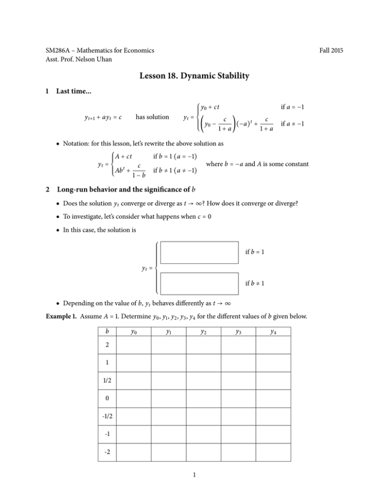
SM286A – Mathematics for Economics
Asst. Prof. Nelson Uhan
Fall 2015
Lesson 18. Dynamic Stability
1
Last time...
y t+1 + ay t = c
has solution
⎧
y0 + ct
⎪
⎪
⎪
⎪
yt = ⎨
c
c
⎪
⎪
)(−a)t +
(y0 −
⎪
⎪
1+a
1+a
⎩
if a = −1
if a ≠ −1
● Notation: for this lesson, let’s rewrite the above solution as
⎧
⎪
if b = 1 (a = −1)
⎪
⎪A + ct
yt = ⎨
where b = −a and A is some constant
c
⎪
⎪
Ab t +
if b ≠ 1 (a ≠ −1)
⎪
⎩
1−b
2
Long-run behavior and the significance of b
● Does the solution y t converge or diverge as t → ∞? How does it converge or diverge?
● To investigate, let’s consider what happens when c = 0
● In this case, the solution is
⎧
⎪
⎪
⎪
⎪
⎪
⎪
⎪
⎪
⎪
⎪
⎪
yt = ⎨
⎪
⎪
⎪
⎪
⎪
⎪
⎪
⎪
⎪
⎪
⎪
⎩
if b = 1
if b ≠ 1
● Depending on the value of b, y t behaves differently as t → ∞
Example 1. Assume A = 1. Determine y0 , y1 , y2 , y3 , y4 for the different values of b given below.
b
y0
y1
y2
2
1
1/2
0
-1/2
-1
-2
1
y3
y4
● From Example 1, we can determine some trends
● When b < 0, y t is
● When b > 0, y t is
● When ∣b∣ < 1, y t is
● When ∣b∣ > 1, y t is
● These trends still hold for different values of A and c
Example 2. Describe the time path given by y t = 5(−1/10)t + 3.
Example 3. Describe the time path described by the difference equation y t+1 + 2y t = 9.
3 The role of A
● If the magnitude of A changes:
● If the sign of A changes:
2