th
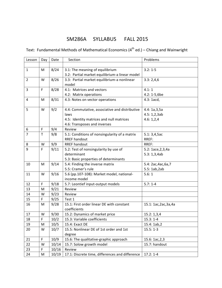
Lesson   Day   Date          Section
1
2
M   8/24   3.1:  The  meaning  of  equilibrium
3.2:    Partial  market  equilibrium-­‐a  linear  model
W   8/26   3.3:    Partial  market  equilibrium-­‐a  nonlinear   model
3
4
5
6
7
8
9
10
11
12
13
14
15
16
17
18
19
20
21
22
23
24
F
M
8/28
8/31
4.1:    Matrices  and  vectors
4.2:    Matrix  operations
4.3:  Notes  on  vector  operations
W   9/2   4.4:  Commutative,  associative  and  distributive   laws
4.5:    Identity  matrices  and  null  matrices
4.6:  Transposes  and  inverses
F   9/4   Review
T   9/8   5.1:  Conditions  of  nonsingularity  of  a  matrix
RREF  handout
W   9/9   RREF  handout
F   9/11   5.2:  Test  of  nonsingularity  by  use  of   determinant
5.3:  Basic  properties  of  determinants
M   9/14   5.4:  Finding  the  inverse  matrix
5.5:  Cramer’s  rule
W   9/16   5.6  (pp.107-­‐108):  Market  model,  national-­‐ income  model
F   9/18   5.7:  Leontief  input-­‐output  models
M   9/21   Review
W   9/23   Review
F   9/25   Test  1
M   9/28   15.1:  First  order  linear  DE  with  constant   coefficients
Problems
3.2:  1-­‐5
3.3:  2,4,6
4.1:  1
4.2:  1-­‐5,6be
4.3:  1acd,
4.4:  1a,3,5a
4.5:  1,2,3ab
4.6:  1,2,4
5.1:  3,4,5ac
RREF:
RREF:
5.2:  1ace,2,3,4a
5.3:  1,3,4ab
5.4:  2ac,4ac,6a,7
5.5:  1ab,2ab
5.6:  1
5.7:  1-­‐4
15.1:  1ac,2ac,3a,4a
W   9/30   15.2:  Dynamics  of  market  price
F   10/2   15.3:  Variable  coefficients
M   10/5   15.4:  Exact  DE
W   10/7   15.5:  Nonlinear  DE  of  1st  order  and  1st
15.2:  1,3,4
15.3:  1-­‐4
15.4:  1ab,2
15.5:  1-­‐3
F   10/9   degree
15.6:  The  qualitative-­‐graphic  approach
W   10/14   15.7:  Solow  growth  model
F   10/16   Review
15.6:  1ac,2,3
15.7:  handout
M   10/19   17.1:  Discrete  time,  differences  and  difference   17.2:  1-­‐4

25
26
27
28
29
30
31
32
33
34
35
36
37
38
39
40   equations
17.2:  Solving  a  1st  order  difference  equation
W   10/21   17.3:  The  dynamic  stability  of  equilibrium
F   10/23   17.4:  The  cobweb  model
M   10/26   Review
W   10/28   Test  2
F   10/30   11.6:  Motivating  examples  :
11.2:  Extreme  values  of  a  function  of  two   variables
M   11/2   11.3:  Determinant  review
Quadratic  forms,  positive/negative   definiteness
W   11/4   11.3:  Second-­‐order  conditions,  the  Hessian
F   11/6   11.4:  Generalization  to  n  variables
M   11/9   11.5:  Convex  and  concave  functions
Convex  sets
F   11/13   11.6:  Solving  the  motivating  examples
M   11/16   Review
W   11/18   12.1:  Effects  of  a  constraint
12.2:  Solving  by  substitution
F   11/20   12.2:  Lagrange  multiplier  method
Shadow  price  interpretation  of  Lagrange   multiplier
M   11/23   12.3:  Second-­‐order  conditions,  the  bordered
Hessian
W   11/25   12.3:  Generalizations:  n  variables  and  1   equality  constraint,  n  variables  and  m  equality   constraints
M   11/30   12.5:  Utility  maximization
12.7:  Least-­‐cost  combination  of  inputs
W   12/2   Review
F   12/4   Review
M   12/7   Test  3
W   12/9   Review
17.3:  1ab,2a,3a
17.4:  2,3
11.2:  1,2
11.3:  1ac,2c
11.3:  3ac,4abe,5abe
11.4:  1-­‐4,5a
11.5:  1-­‐6
11.6:  1-­‐3
12.2:  1-­‐3
12.3:  1
12.5:  handout
12.7:  handout
41
42
43
44
Student  Learning  Outcomes:  Learning  Goals  and  Objectives  for  Mathematics  for  Economics  (SM286A):
Upon  successful  completion  of  this  course,  students  are  able  to  do  the  following:
1.
2.
3.
4.
Perform  basic  operations  with  matrices.
Solve  simple  equilibrium  models  in  economics  using  matrix  methods.
Apply  the  theory  of  first  order  differential  equations  and  difference  equations  to  analyze   growth  models  in  economics.
Apply  the  theory  of  constrained  optimization  to  problems  involving  utility  maximization  or   least-­‐cost  combination  of  inputs.