Ralph’s Solver Training
by Anil Arya and Richard A. Young
Ralph wants you to help him solve two mathematical programming problems using Excel. For Problem 1, he has provided
detailed instructions for you to follow.
Problem 1:
Max
subject to:
6 x1 + 2 x2
2 x1 +
x2 ≤ 100
x1 + 3 x2 ≤ 120
x1, x2
≥ 0
Below are Ralph’s instructions.
Note: These instructions accompany Excel 2007. Some minor differences exist for later versions.
A.
1.
2.
3.
B.
1.
2.
3.
Setting Up the Parameters in the Spreadsheet:
Start up Excel. Open up a new spreadsheet.
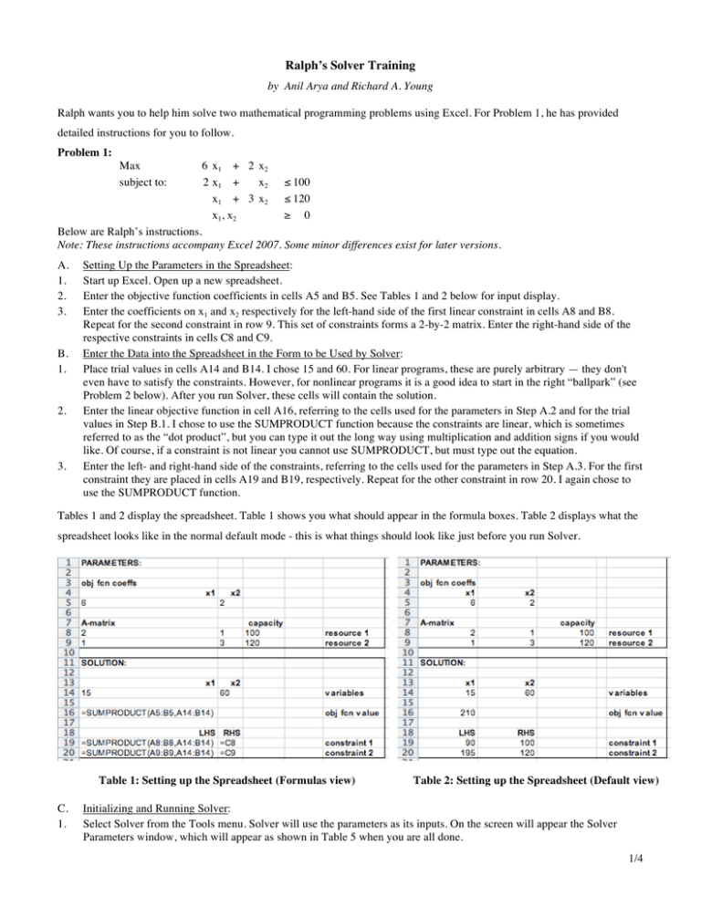
Enter the objective function coefficients in cells A5 and B5. See Tables 1 and 2 below for input display.
Enter the coefficients on x1 and x2 respectively for the left-hand side of the first linear constraint in cells A8 and B8.
Repeat for the second constraint in row 9. This set of constraints forms a 2-by-2 matrix. Enter the right-hand side of the
respective constraints in cells C8 and C9.
Enter the Data into the Spreadsheet in the Form to be Used by Solver:
Place trial values in cells A14 and B14. I chose 15 and 60. For linear programs, these are purely arbitrary — they don't
even have to satisfy the constraints. However, for nonlinear programs it is a good idea to start in the right “ballpark” (see
Problem 2 below). After you run Solver, these cells will contain the solution.
Enter the linear objective function in cell A16, referring to the cells used for the parameters in Step A.2 and for the trial
values in Step B.1. I chose to use the SUMPRODUCT function because the constraints are linear, which is sometimes
referred to as the “dot product”, but you can type it out the long way using multiplication and addition signs if you would
like. Of course, if a constraint is not linear you cannot use SUMPRODUCT, but must type out the equation.
Enter the left- and right-hand side of the constraints, referring to the cells used for the parameters in Step A.3. For the first
constraint they are placed in cells A19 and B19, respectively. Repeat for the other constraint in row 20. I again chose to
use the SUMPRODUCT function.
Tables 1 and 2 display the spreadsheet. Table 1 shows you what should appear in the formula boxes. Table 2 displays what the
spreadsheet looks like in the normal default mode - this is what things should look like just before you run Solver.
Table 1: Setting up the Spreadsheet (Formulas view)
C.
1.
Table 2: Setting up the Spreadsheet (Default view)
Initializing and Running Solver:
Select Solver from the Tools menu. Solver will use the parameters as its inputs. On the screen will appear the Solver
Parameters window, which will appear as shown in Table 5 when you are all done.
1/4
2.
3.
4.
5.
Place the cursor in the Set Target Cell box and click on cell A16. This is a maximization problem, so make sure Max is
selected.
Type A14:B14 in By Changing Cells box or place the curser in the box and drag your mouse over the cells.
To build the constraints click Add. The Add Constraint window will appear as in Table 3. Type A19 in the Cell
Reference box. The direction of the inequality should be set at <= for the first constraint. Type B19 in the Constraint:
box. Click Add to keep adding constraints. You also can drag down to enter the left- and right hand sides, but the
inequalities must all go in the same direction – this is what is shown in Table 3. A blank Add Constraint window will
reappear. To stop adding constraints click OK.
From the Solver Parameters window (Table 5) select the Options box, which will appear as in Table 4). Then select
Assume Linear Model (this will make the program run more efficiently). For this problem you should select Assume
Non-Negative – this is important, and it may be in the Table 5 window in later versions of Excel. Click Okay to return to
the Solver box.
Table 3: Add Constraint Window
Table 4: Solver Options Window
Table 5: Solver Window for Completely Specified Model
2/4
6.
Table 5 displays the Solver window for the model. Note the software has inserted dollar signs in cell labels; you did not
need to do that yourself. Now you are ready to solve the LP. Click Solve. If the solution looks a little messy, run Solver
again, with the current solution as the starting solution.
Table 6: Results Window for Solver
D.
1.
2.
Sensitivity Analysis:
If you've done everything okay, a window should appear with the message "Solver found a solution. All constraints and
optimality conditions are satisfied." (See Table 6 above.) Alternatively, you may get a message indicating that you need
to run more iterations. This is unlikely with an LP of the size we'll be dealing with, but may occur if you run a non-linear
program (see Problem 2 below). If this happens, click “OK” and then select Solve again, with the current solution as the
starting solution. If you get a more troublesome message, such as “the problem has not converged,” etc., you probably
have entered the problem incorrectly. Make sure that it's maximizing if that's what you want to do. Check you have
entered the objective function and constraints correctly. Make sure the direction of the inequalities is correct. Make sure
you have chosen Assume Non-Negative.
Try selecting from within the Reports section of the Solver Results window one or more of: Answer, Sensitivity, and
Limits. For example, if you select Sensitivity, a window will appear as in Table 7 below. This report is automatically
placed into a separate Excel Sheet titled “Sensitivity Report”. You see the “shadow prices” are 3 on the first resource
constraint and zero on the second. We will talk about shadow prices quite a bit in this course, and you will continue to do
so in BUS-ADM MGT 331 and BUS-ADM MGT 630.
Table 7: Results of Sensitivity Analysis
3.
Now click on “Sheet 1”, which will appear as in Table 8 below. The optimal solution is: x1 = 50, x2 = 0, and the objective
function is 5,000. Well done!
3/4
Table 8: Successfully Run Program
Problem 2:
This one is based on Examples 2.2 and 2.6 in Demski, Managerial Uses of Accounting Information. It will be helpful to you
when we get to chapter 2.
Min
5 z1 + 20 z2
subject to:
z1z 2
≥ q
z1 ≤ 15
z1, z2 ≥ 0
!
Try running the example for six cases: q = {0, 5, 10, 15, 20, 25}. This involves running solver six times. Don’t forget to extract
the shadow prices for each case. What do you observe?
Solver hints:
(1) notice this is a minimization problem
(2) because of the square root in the first constraint, you probably should try positive values for your starting solution.
(3) in the previous example Assume Linear Model was selected, because that was a linear program. For this nonlinear
program, you should go into Options and make sure you have not selected Assume Linear Model. The other options are
normally fine to leave at their default settings.
(4) when you enter the left hand side of the first constraint into the objective function cell you will want to make use of the
SQRT function under the Insert menu, or type in “(z1 z2)^(1/2)”.
4/4