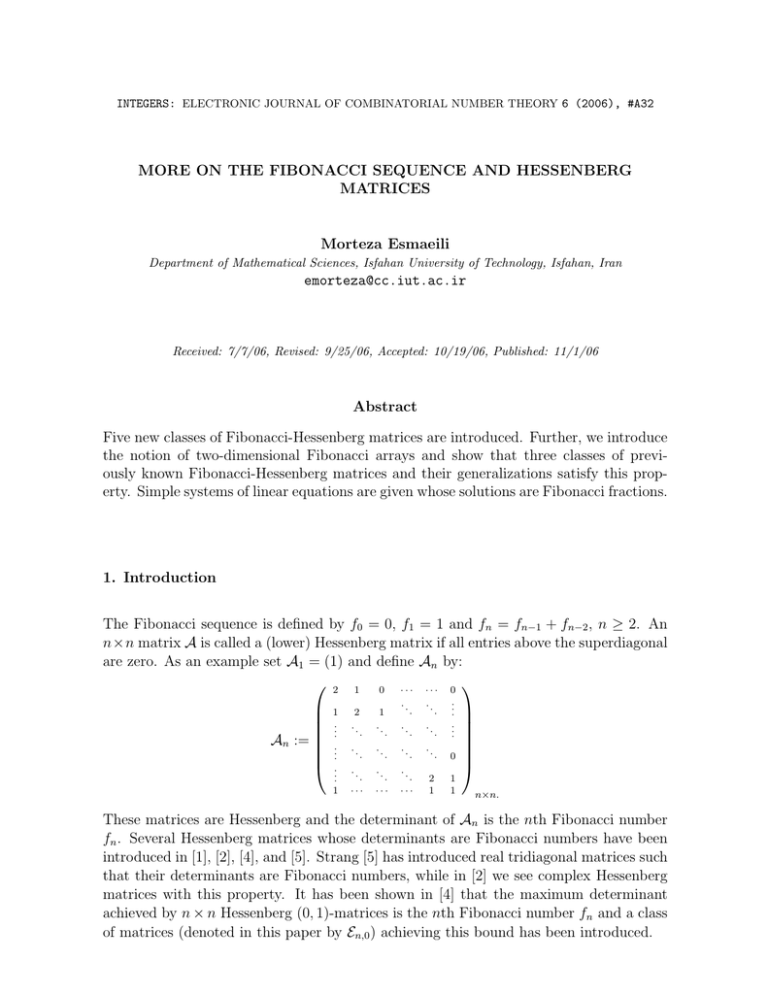
INTEGERS: ELECTRONIC JOURNAL OF COMBINATORIAL NUMBER THEORY 6 (2006), #A32
MORE ON THE FIBONACCI SEQUENCE AND HESSENBERG
MATRICES
Morteza Esmaeili
Department of Mathematical Sciences, Isfahan University of Technology, Isfahan, Iran
emorteza@cc.iut.ac.ir
Received: 7/7/06, Revised: 9/25/06, Accepted: 10/19/06, Published: 11/1/06
Abstract
Five new classes of Fibonacci-Hessenberg matrices are introduced. Further, we introduce
the notion of two-dimensional Fibonacci arrays and show that three classes of previously known Fibonacci-Hessenberg matrices and their generalizations satisfy this property. Simple systems of linear equations are given whose solutions are Fibonacci fractions.
1. Introduction
The Fibonacci sequence is defined by f0 = 0, f1 = 1 and fn = fn−1 + fn−2 , n ≥ 2. An
n×n matrix A is called a (lower) Hessenberg matrix if all entries above the superdiagonal
are zero. As an example set A1 = (1) and define An by:
 2 1 0 ··· ··· 0 



An := 



1
.
..
..
.
.
.
.
1
2
..
..
..
.
1
..
.
..
.
···
..
..
.
..
.
..
.
···
..
.
..
.
.
..
.
.
..
.
..
.
..
.
0
.
···
2
1
1
1







n×n.
These matrices are Hessenberg and the determinant of An is the nth Fibonacci number
fn . Several Hessenberg matrices whose determinants are Fibonacci numbers have been
introduced in [1], [2], [4], and [5]. Strang [5] has introduced real tridiagonal matrices such
that their determinants are Fibonacci numbers, while in [2] we see complex Hessenberg
matrices with this property. It has been shown in [4] that the maximum determinant
achieved by n × n Hessenberg (0, 1)-matrices is the nth Fibonacci number fn and a class
of matrices (denoted in this paper by En,0 ) achieving this bound has been introduced.
INTEGERS: ELECTRONIC JOURNAL OF COMBINATORIAL NUMBER THEORY 6 (2006), #A32
2
In this paper, we consider sequences of Hessenberg matrices whose determinants are
in the form tfn−1 +fn−2 or fn−1 +tfn−2 for some real or complex number t. Such matrices
will be referred to as Fibonacci-Hessenberg matrices.
In Section 2 we introduce five new classes of Fibonacci-Hessenberg matrices. As a new
concept, the two-dimensional Fibonacci array is introduced in Section 3. Three classes
of Fibonacci-Hessenberg matrices satisfying this property are given.
2. More Fibonacci-Hessenberg Matrices
As mentioned above, several connections between the Fibonacci sequence and Hessenberg
matrices have been given in [1], [2], [4], and [5]. In this section we develop some of these
connections and provide more examples.
The Fibonacci recurrence relation an = an−1 + an−2 beginning with a1 = 1 and a2 = t
produces the sequence 1, t, t + 1, 2t + 1, 3t + 2, 5t + 3, · · ·. Thus an = tfn−1 + fn−2 for
n ≥ 1 and an = fn if and only if t = 1. On the other hand, the sequence an = an−1 + an−2
starting at a1 = t and a2 = 1 satisfies an = tfn−2 + fn−1 .
Definition 1 Given a real or complex number t and an integer n, we refer to numbers
tfn−1 + fn−2 and fn−1 + tfn−2 as type 1 and type 2, respectively, (t, n)-Fibonacci, briefly
t-Fibonacci, numbers. A sequence of Hessenberg matrices A1 , A2 , A3 , · · ·, where An is
an n × n matrix, is defined to be a Fibonacci-Hessenberg matrix if there exists an integer
m > 0 and a number t such that, for each n ≥ m, the determinant of An is a t-Fibonacci
number and such that the determinants are of the same type.
Example 1 Given a number t, let Rn,t denote the n × n matrix given below.

Rn,t



:= 



2
1
0
1
..
.
.
..
.
..
1
2
..
.
1
..
.
..
.
..
..
.
···
..
.
.
···
···
..
.
..
.
..
.
..
.
···
···
..
.
..
.
..
.
0
2
1
1
t+1
0
..
.
..
.








n×n.
The determinant of Rn,t is denoted by rn,t . It can be shown that rn,t = tfn+1 + fn , n ≥ 1,
(see relation (10) in the proof of Theorem 2) and hence Rn,t is a Fibonacci-Hessenberg
matrix. Thus, for instance, rn,−1 = −fn+1 + fn = −fn−1 ; that is rn,−1 generates the
additive inverse of the Fibonacci sequence. The Lucas numbers are defined by l1 = 1,
l2 = 3 and ln = ln−1 + ln−2 for n > 2. One can easily verify by induction that ln =
fn−1 + fn+1 . Hence rn,3 = 3fn+1 + fn = fn+1 + fn+3 = ln+2 . For t = 0 we have rn,0 = fn ,
INTEGERS: ELECTRONIC JOURNAL OF COMBINATORIAL NUMBER THEORY 6 (2006), #A32
3
Table 1: Determinant rn,t for 1 ≤ n ≤ 5 and t = −1, 0, 1, 2, 3.
t\n
3
2
1
0
−1
1 2
3
4
4 7 11 18
3 5
8 13
2 3
5
8
1 1
2
3
0 −1 −1 −2
5
29
21
13
5
−3
while rn,1 = fn+1 + fn = fn+2 and rn,2 = 2fn+1 + fn = fn+3 . These are illustrated by
Table 1.
Given a positive integer n, let Cn,t be the n × n matrix in which the entries below the
diagonal are 1, the lowest entry of the nth column is t + 1 and the other diagonal entries
are 2, the entries on the superdiagonal are −1 and the entries above the superdiagonal
are zero. Changing the first element of the first column in Cn,t to 2, we get another
Hessenberg matrix denoted by Bn,t . Matrices C5,t and B5,t are given below.
 2 −1 0 0
 1 −1 0 0


0
0
C5,t := 
1
1
1
1
2
1
1
1
−1
2
1
1
0
−1
2
1
0
0
−1
t+1
 B5,t := 
1
1
1
1
2
1
1
1
−1
2
1
1
0
−1
2
1
0
0
−1
t+1

Proposition 1 The determinant of Cn,t , denoted cn,t , is cn,t = f2n + tf2n−1 , n ≥ 1, and
Bn,t has determinant bn,t = f2n−1 + tf2n−2 , n ≥ 1.
Proof. We prove the statements by induction on n. It is obvious that these statements
hold for n = 1, 2. Suppose n ≥ 3. By the cofactor expansion along the first row we get
cn,t = 2cn−1,t + bn−1,t and bn,t = cn−1,t + bn−1,t . It follows from these two relations that
bn,t = cn,t − cn−1,t .
(1)
Relations (1) and cn,t = 2cn−1,t + bn−1,t imply that cn,t = 3cn−1,t − cn−2,t . Using the
induction hypothesis we get
cn,t = 3cn−1,t − cn−2,t
= 3(f2n−2 + tf2n−3 ) − (f2n−4 + tf2n−5 )
= (3f2n−2 − f2n−4 ) + t(3f2n−3 − f2n−5 )
= f2n + tf2n−1 .
Finally, it follows from bn,t = cn,t − cn−1,t and cn,t = f2n + tf2n−1 that
bn,t = f2n−1 + tf2n−2 .
!
The three classes of Fibonacci-Hessenberg matrices given above are generalizations of
matrices Dn , Cn , and Bn introduced in [1]. In fact the matrices Dn , Cn , and Bn given in
[1] are Rn,1 , Cn,1 , and Bn,1 , respectively.
INTEGERS: ELECTRONIC JOURNAL OF COMBINATORIAL NUMBER THEORY 6 (2006), #A32
4
Now we introduce five new classes of Fibonacci-Hessenberg matrices. Given a number
t, let Kn,t be the n × n Hessenberg matrix in which the superdiagonal entries are −1,
the entry located on the nth row and nth column is t + 1 and the other diagonal entries
are 2, and the entries on each column and below the diagonal are alternately −1 and 1
starting with −1. The matrix K5,t is given by (2).
Replacing the top-left entry (the entry located in the first row and first column) in
Kn,t with 1, we obtain another Hessenberg matrix denoted by Ln,t . Replacing the superdiagonal entries in both Kn,t and Ln,t with 1, two more classes of Hessenberg matrices,
denoted Kn,t and Ln,t , respectively, are obtained.

K5,t = 

K5,t = 
2
−1
1
−1
1
−1
2
−1
1
−1
0
−1
2
−1
1
0
0
−1
2
−1
0
0
0
−1
t+1
2
−1
1
−1
1
1
2
−1
1
−1
0
1
2
−1
1
0
0
1
2
−1
0
0
0
1
t+1




 L5,t = 
 L5,t = 
1
−1
1
−1
1
−1
2
−1
1
−1
0
−1
2
−1
1
0
0
−1
2
−1
0
0
0
−1
t+1
1
−1
1
−1
1
1
2
−1
1
−1
0
1
2
−1
1
0
0
1
2
−1
0
0
0
1
t+1



(2)

Theorem 1 Let kn,t , ln,t , k n,t and ln,t denote the determinants of Kn,t , Ln,t , Kn,t and
Ln,t , respectively. Then

kn,t = fn + tfn+1 , n ≥ 1;






+


l1,t = t + 1,




ln,t = kn−2,t = fn−2 + tfn−1 , n ≥ 2;



k n,t = f2n + tf2n−1 , n ≥ 1;






+


l1,t = 1 + t,



ln,t = k n−1,t + ln−1,t = f2n−1 + tf2n−2 , n ≥ 2.
Therefore, the four introduced classes of Hessenberg matrices are indeed FibonacciHessenberg matrices.
Proof. The proof is by induction on n. Due to the similarity between matrices Kn,t (Ln,t )
and Kn,t (resp. Ln,t ), we just prove the first two statements. It is easily verified that the
statements hold for 1 ≤ n ≤ 3. Assume that n ≥ 4. Using cofactor expansion along the
first row we obtain:
+
n ≥ 4;
ln,t = kn−1,t − ln−1,t ,
(3)
kn,t = 2kn−1,t − ln−1,t ,
n ≥ 4.
Therefore,
ln,t = kn−1,t − ln−1,t
= (2kn−2,t − ln−2,t ) − (kn−2,t − ln−2,t )
(4)
= kn−2,t .
INTEGERS: ELECTRONIC JOURNAL OF COMBINATORIAL NUMBER THEORY 6 (2006), #A32
5
Relations (3) and (4) imply
kn,t = 2kn−1,t − ln−1,t = 2kn−1,t − kn−3,t ,
n ≥ 4.
(5)
This, together with the induction hypothesis, result in:
kn,t = 2kn−1,t − kn−3,t = 2 (fn−1 + tfn ) − (fn−3 + tfn−2 )
= (fn−1 + fn−1 − fn−3 ) + (tfn + tfn − tfn−2 )
= (fn−1 + fn−2 + fn−3 − fn−3 ) + (tfn + tfn−1 + tfn−2 − tfn−2 )
= fn + tfn+1 .
!
,
1
1
Define E1,t = (t + 1) and E2,t = 0 t + 1 . Given the n × n matrix En,t , a new matrix
En+1,t is formed by adding one row of weight one and starting with 1 to the top of En,t
and then adding a new column with alternating 1’s and 0’s, starting with a 1, to the left
of the obtained matrix. The matrix E5,t is given below. The matrix En,0 was introduced
in [4] and it was shown in [4] that the determinant of En,0 , n ≥ 1, is fn . Let i denote
the usual complex unit with i2 = −1. Replacing the entry of En,t located in the ith row
and (i + 1)th column, 1 ≤ i < n, with (−1)i+n i, we obtain another Hessenberg matrix
denoted by Hn,t . The matrix H5,t is shown below.
 1 1 0 0 0 
 1 i 0 0 0 
E5,t = 
0
1
0
1
1
0
1
0
1
1
0
1
0
1
1
0
0
0
1
t+1
 H5,t = 
0
1
0
1
1
0
1
0
−i
1
0
1
0
i
1
0
0
0
−i
t+1

Proposition 2 The determinants of En,t and Hn,t , denoted by en,t and hn,t , respectively,
are e1,t = h1,t = t + 1 and en,t = hn,t = tfn−1 + fn for n ≥ 2. Thus En,t and Hn,t are
Fibonacci-Hessenberg matrices.
Proof. Consider Hn,t . Obviously we have h1,t = h2,t = t + 1 and h3,t = 2t + 3. Suppose
#
n ≥ 4 and that the statement holds for each integer 0 < m < n. Let Hn,t
be the
matrix obtained from Hn,t by means of deleting the first row and second column. It
#
is easy to see that using cofactor expansion along the first row on both Hn,t and Hn,t
results in hn,t = hn−1,t + hn−2,t . Therefore, it follows from the induction hypothesis that
hn,t = hn−1,t + hn−2,t = (tfn−2 + fn−1 ) + (tfn−3 + fn−2 ) = tfn−1 + fn . The same argument
!
applies to En,t .
3. Two-dimensional Fibonacci Arrays
From among the introduced Fibonacci matrices, the matrices Rn,t , Cn,t and En,t have a
further interesting property. Given an n × n matrix M, let M(i) be the matrix obtained
from M by replacing its ith column with the all one column vector 1. The mentioned
(i)
(i)
matrices have the property that the determinants of their associated matrices Rn,t , Cn,t
6
INTEGERS: ELECTRONIC JOURNAL OF COMBINATORIAL NUMBER THEORY 6 (2006), #A32
(i)
and En,t , 1 ≤ i ≤ n, are t-Fibonacci numbers. This leads to a connection between
Fibonacci fractions and the all one vector 1.
(i)
(i)
(i)
(i)
(i)
(i)
Theorem 2 Let rn,t , cn,t and en,t be determinants of Rn,t , Cn,t and En,t , respectively.
Then we have
 (i)

rn,t = tfn−i + fn−i−1 , n ≥ i ≥ 1;


.

(i)

rn,t = t + ni=1 rn,t ;







(i)


+ tf
, n ≥ i ≥ 1;
 cn,t = f2(n−i)+1
.n (i) 2(n−i)
(6)
cn,t = t + i=1 cn,t ;





(1)
(1)


e1,t = 1; en,t = tfn−3 + fn−2 , n ≥ 2;



(i)


en,t = tfn−i + fn−i+1 , n ≥ i ≥ 2;


.

(i)
2en,t = (t + 1) + ni=1 en,t , n ≥ 2.
Proof. We use induction on n to prove the statements related to the Fibonacci-Hessenberg
matrices Rn,t ; similar arguments apply to the other two classes of matrices. Setting f0 = 0
and f−1 = 1, it is easy to verify that the statements hold for 1 ≤ n ≤ 3. Evaluating
(1)
the determinants of matrices Rn,t and Rn,t by cofactor expansion along the first row, we
have
/
(1)
(1)
n ≥ 3;
rn,t = rn−1,t − rn−1,t ,
(7)
(1)
rn−1,t = 2rn−2,t − rn−2,t ,
n ≥ 3.
Therefore,
(1)
(1)
rn,t = r,n−1,t − rn−1,t - ,
(1)
(1)
= 2rn−2,t − rn−2,t − rn−2,t − rn−2,t
= rn−2,t .
(8)
It follows from (7) and (8) that
(1)
rn,t = 2rn−1,t − rn−1,t = 2rn−1,t − rn−3,t ,
n ≥ 3.
(9)
This together with the induction hypothesis result in
rn,t = 2rn−1,t − rn−3,t
= 2 (tfn + fn−1 ) − (tfn−2 + fn−3 )
= t(2fn − fn−2 ) + (2fn−1 − fn−3 )
= tfn+1 + fn ,
and hence
(10)
(1)
rn,t = rn−2,t = tfn−1 + fn−2 .
(11)
(i)
(i−1)
By cofactor expansion along the first row, one can easily verify that rn,t = rn−1,t if
2 ≤ i ≤ n − 1, and thus
(i)
rn,t = rn−i−1,t = tfn−i + fn−i−1 ,
2 ≤ i ≤ n − 1.
(12)
7
INTEGERS: ELECTRONIC JOURNAL OF COMBINATORIAL NUMBER THEORY 6 (2006), #A32
The augmented matrices obtained from a given matrix M by adding the all one column
vector 1 to the left and the right of M are denoted by 1M and M1, respectively.
(n)
Evaluating the determinants by using cofactors along the first row, we obtain rn,t =
(n−1)
(n−1)
2rn−1,t + (−1)n+1 det(1M) where M1 is the matrix Rn−1,t . Therefore,
(n)
(n−1)
(n−1)
(n−1)
(13)
rn,t = 2rn−1,t + (−1)2n−1 rn−1,t = rn−1,t = 1 = tf0 + f−1 .
.
It is easily checked by induction on n that nj=−1 fj = fn+2 . This together with the
.
(i)
(i)
equations rn,t = tfn+1 + fn and rn,t = tfn−i + fn−i−1 imply that rn,t = t + ni=1 rn,t . !
Corollary 1 (Fibonacci Fractions and Hessenberg Matrices) The system of equations
Rn,t x = 1 has the unique solution
xi =
fn−i−1 + tfn−i
, 1 ≤ i ≤ n.
fn + tfn+1
(14)
Similarly, the system of equations Cn,t x = 1 has the solution
xi =
We also have x1 =
En,t x = 1.
tfn−3 +fn−2
tfn−1 +fn
f2(n−i)+1 + tf2(n−i)
, 1 ≤ i ≤ n.
f2n + tf2n−1
and xi =
tfn−i +fn−i+1
,
tfn−1 +fn
(15)
2 ≤ i ≤ n, as the unique solution of
Proof. It follows from (6) and Cramer’s rule that the system Rn,t x = 1 has unique
r
(i)
+tfn−i
n,t
= fn−i−1
, 1 ≤ i ≤ n. The same argument applies to the systems
solution xi = rn,t
fn +tfn+1
Cn,t x = 1 and En,t x = 1.
!
In particular, according to (14), for t = 0, 1, 2 the system Rn,t x = 1 has solutions:

fn−i−1
t = 0;

 x i = fn ,
fn−i +fn−i−1
fn−i+1
xi = fn+1 +fn = fn+2 , t = 1;

 x = 2fn−i +fn−i−1 = fn−i+2 , t = 2.
i
2fn+1 +fn
fn+3
It also follows from (15) that for t = 0, 1, 2 the system Cn,t x = 1 has solutions

f2(n−i)+1

t = 0;

 xi = f2n ,
xi =


 xi =
f2(n−i+1)
,
f2n+1
f2(n−i+1) +f2(n−i)
,
f2n+1 +f2n−1
t = 1;
t = 2.
(i)
Consider the n × n Fibonacci-Hessenberg matrix Rn,t . For 1 ≤ i ≤ n we have rn,t =
tfn−i + fn−i+1 . This t-Fibonacci number depends on both n and i, and hence we have a
two-dimensional array r(n, i; t) of t-Fibonacci numbers.
INTEGERS: ELECTRONIC JOURNAL OF COMBINATORIAL NUMBER THEORY 6 (2006), #A32
8
(i)
Table 2: The Values of rn,t for 1 ≤ n, i ≤ 6.
n\i
1
2
3
4
5
6
1
tf0 + f−1
tf1 + f0
tf2 + f1
tf3 + f2
tf4 + f3
tf5 + f4
2
3
4
5
tf0 + f−1
tf1 + f0
tf2 + f1
tf3 + f2
tf4 + f3
tf0 + f−1
tf1 + f0
tf2 + f1
tf3 + f2
tf0 + f−1
tf1 + f0
tf2 + f1
tf0 + f−1
tf1 + f0
6
tf0 + f−1
(i)
Table 3: The Values of rn,1 for 1 ≤ n, i ≤ 6.
n\i
1
2
3
4
5
6
1
1
1
2
3
5
8
2
3
4
5
6
1
1
2
3
5
1
1
2
3
1
1
2
1
1
1
Table 2 represents r(n, i; t) for 1 ≤ n, i ≤ 6. Asymptotically, all rows and columns of
the array r(n, i; t) are the same. Table 3 represents r(n, i; 1) for 1 ≤ n, i ≤ 6. For a fixed
n the nth row of the array consists of the first n Fibonacci numbers and, for each i, the
ith column, starting at the ith entry, is also the Fibonacci sequence.
In the context of systems theory [3], we may consider the determinant function as an
(i)
operator and interpret r(n, i; t) = Det(Rn,t ) as a two-dimensional system. The results
show that this system is invariant in the sense that its output is always a t-Fibonacci
number. We can also say that the system is invariant with respect to fixing any of the
two variables n and i; that is, its output with a fixed n is identical to the output when i
is fixed and n varies.
References
[1] N.D. Cahill, J.R. D! Errico, D.A. Narayan and J.Y. Narayan, “Fibonacci Determinants,” The College Math. Journal of The Math. Association of America, vol. 33, no. 3, pp. 221–225, May 2002.
[2] N.D. Cahill, J.R. D! Errico, J. Spence, “Complex factorizations of the Fibonacci and Lucas numbers,” Fibonacci Quarterly, vol. 41, no. 1, pp. 13–19, Feb. 2003.
[3] K.B. Datta and B. M. Mohan, Orthogonal Functions in Systems and Control, IIT, Kharagpur,
India, 1995.
[4] Ching Li,“The Maximum Determinant of an nxn Lower Hessenberg (0,1) matrix,” Linear Algebra
and Its Applications, 183, pp. 147–153, 1993.
[5] G. Strang, Introduction to Linear Algebra, 2nd Edition, Wellesley MA, Wellesley-Cambridge, 1998.