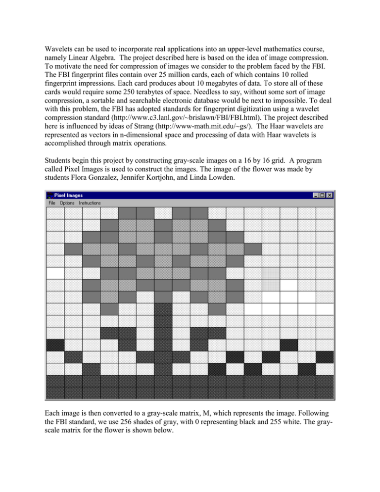
Wavelets can be used to incorporate real applications into an upper-level mathematics course,
namely Linear Algebra. The project described here is based on the idea of image compression.
To motivate the need for compression of images we consider to the problem faced by the FBI.
The FBI fingerprint files contain over 25 million cards, each of which contains 10 rolled
fingerprint impressions. Each card produces about 10 megabytes of data. To store all of these
cards would require some 250 terabytes of space. Needless to say, without some sort of image
compression, a sortable and searchable electronic database would be next to impossible. To deal
with this problem, the FBI has adopted standards for fingerprint digitization using a wavelet
compression standard (http://www.c3.lanl.gov/~brislawn/FBI/FBI.html). The project described
here is influenced by ideas of Strang (http://www-math.mit.edu/~gs/). The Haar wavelets are
represented as vectors in n-dimensional space and processing of data with Haar wavelets is
accomplished through matrix operations.
Students begin this project by constructing gray-scale images on a 16 by 16 grid. A program
called Pixel Images is used to construct the images. The image of the flower was made by
students Flora Gonzalez, Jennifer Kortjohn, and Linda Lowden.
Each image is then converted to a gray-scale matrix, M, which represents the image. Following
the FBI standard, we use 256 shades of gray, with 0 representing black and 255 white. The grayscale matrix for the flower is shown below.
240


240


240



240


240


255



240


240



240


240


240



 50


240


240



 75


 75
240
240
240
130
130
240
130
130
240
240
240
240
240
240
240
240
130
175
175
130
175
175
130
240
240
240
240
240
240
130
130
175
175
130
175
175
130
130
240
240
240
240
130
175
175
130
175
175
175
130
175
175
130
240
240
240
240
130
175
175
130
175
130
175
175
130
240
240
240
240
240
240
130
130
175
175
175
130
130
240
240
225
240
240
240
130
175
175
130
130
130
175
175
130
240
225
255
240
240
130
175
130
240
130
240
130
175
130
240
255
255
255
240
240
130
240
240
75
240
240
130
240
255
255
255
255
240
240
240
240
240
75
240
240
240
240
240
240
240
240
240
240
75
75
240
75
240
75
75
240
240
240
240
240
240
240
240
75
240
75
240
75
240
240
240
240
50
240
75
240
240
240
75
75
75
240
240
50
240
50
240
240
240
75
240
240
240
75
240
240
50
240
50
240
240
50
75
75
75
75
75
75
75
75
75
75
75
75
75
75
75
75
75
75
75
75
75
75
75
75
75
75
75
75
240


240

240


240


240

240


240

240


255


240

240


240


50

240


75

75
Throughout the course, we discuss how wavelets are used to process this kind of data. The ideas
that are needed to understand the process are matrix multiplication, how to solve systems of
linear equations, matrix inverses, linear combinations, linear dependence and independence,
bases, and how to identify piecewise constant functions with vectors in n-space. Through these
discussions, students learn how to process their gray-scale matrices using matrices. Specifically,
they construct the 16 by 16 wavelet matrix A:
1


1


1



1


1


1



1


1



1


1


1



1


1


1



1


1
1
1
0
1
0
0
0
1
0
0
0
0
0
0
1
1
0
1
0
0
0
-1
0
0
0
0
0
0
1
1
0
-1
0
0
0
0
1
0
0
0
0
0
1
1
0
-1
0
0
0
0
-1
0
0
0
0
0
1
-1
0
0
1
0
0
0
0
1
0
0
0
0
1
-1
0
0
1
0
0
0
0
-1
0
0
0
0
1
-1
0
0
-1
0
0
0
0
0
1
0
0
0
1
-1
0
0
-1
0
0
0
0
0
-1
0
0
0
-1
0
1
0
0
1
0
0
0
0
0
1
0
0
-1
0
1
0
0
1
0
0
0
0
0
-1
0
0
-1
0
1
0
0
-1
0
0
0
0
0
0
1
0
-1
0
1
0
0
-1
0
0
0
0
0
0
-1
0
-1
0
-1
0
0
0
1
0
0
0
0
0
0
1
-1
0
-1
0
0
0
1
0
0
0
0
0
0
-1
-1
0
-1
0
0
0
-1
0
0
0
0
0
0
0
-1
0
-1
0
0
0
-1
0
0
0
0
0
0
0
0


0

0


0


0

0


0

0


0


0

0


0


0

0


1

-1
The wavelet coefficients for their images are found by solving the matrix equation AX = M.
Since A is invertible, this equation is easily solved with Maple. Once the wavelet coefficients are
found, do hard thresholding to achieve further compression. They then de-process the data to see
what the reconstructed image will look like. With a threshold level of 6, the reconstructed flower
image looks like
We think this project is an excellent example of how the ideas students meet in linear algebra are
used in the "real world" and our students have responded positively to the experience.
For more information contact us at :
Ed Aboufadel (aboufade@gvsu.edu)
Steve Schlicker (schlicks@gvsu.edu)
Department of Mathematics and Statistics
Grand Valley State University
Allendale, MI 49401