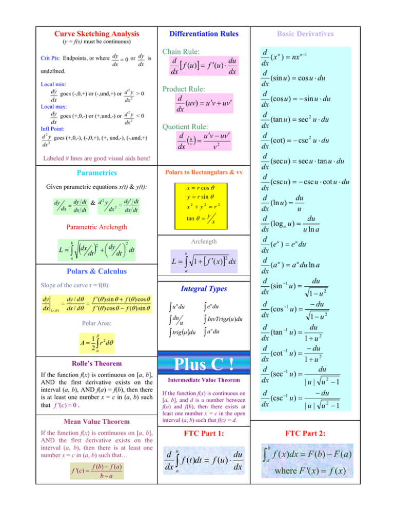
Curve Sketching Analysis
Basic Derivatives
Differentiation Rules
(y = f(x) must be continuous)
Crit Pts: Endpoints, or where dy = 0 or dy is
dx
dx
undefined.
Local min:
dy goes (-,0,+) or (-,und,+) or d 2 y > 0
dx
dx 2
Local max:
dy goes (+,0,-) or (+,und,-) or d 2 y < 0
dx
dx 2
Infl Point:
d 2 y goes (+,0,-), (-,0,+), (+, und,-), (-,und,+)
dx 2
Chain Rule:
d
[ f (u )] = f ′(u ) ⋅ du
dx
dx
Product Rule:
d
(uv) = u ′v + uv ′
dx
Quotient Rule:
d u
( v ) = u ′v −2 uv ′
dx
v
Labeled # lines are good visual aids here!
Polars to Rectangulars & vv
Parametrics
Given parametric equations x(t) & y(t):
dy
dx
x = r cos θ
y = r sin θ
dy ′ dt
dy dt & d 2 y
2 =
dx
dx dt
dx dt
=
x2 + y2 = r2
tan θ = y
x
Parametric Arclength
b
L=∫
a
(dx dt ) + ⎛⎜⎝ dy dt ⎞⎟⎠ dt
2
Arclength
2
Polars & Calculus
b
L = ∫ 1 + [ f ′( x)] dx
a
Slope of the curve r = f(θ):
dy
dx
( r ,θ )
dy / dθ
f ′(θ ) sin θ + f (θ ) cos θ
=
=
dx / dθ
f ′(θ ) cos θ − f (θ ) sin θ
Polar Area:
2
Integral Types
∫ e du
∫ u du
∫ InvTrigs(u)du
∫ du u
∫ trig (u )du ∫ a du
n
u
u
β
A=
1 2
r dθ
2 α∫
Rolle’s Theorem
If the function f(x) is continuous on [a, b],
AND the first derivative exists on the
interval (a, b), AND f(a) = f(b), then there
is at least one number x = c in (a, b) such
that f '(c) = 0 .
Mean Value Theorem
If the function f(x) is continuous on [a, b],
AND the first derivative exists on the
interval (a, b), then there is at least one
number x = c in (a, b) such that…
f '(c) =
f (b) − f (a)
b−a
Plus C !
Intermediate Value Theorem
If the function f(x) is continuous on
[a, b], and d is a number between
f(a) and f(b), then there exists at
least one number x = c in the open
interval (a, b) such that f(c) = d.
d n
( x ) = nx n −1
dx
d
(sin u ) = cos u ⋅ du
dx
d
(cos u ) = − sin u ⋅ du
dx
d
(tan u ) = sec 2 u ⋅ du
dx
d
(cot) = − csc 2 u ⋅ du
dx
d
(sec u ) = sec u ⋅ tan u ⋅ du
dx
d
(csc u ) = − csc u ⋅ cot u ⋅ du
dx
d
du
(ln u ) =
dx
u
d
du
(log a u ) =
dx
u ln a
d u
(e ) = e u du
dx
d u
(a ) = a u du ln a
dx
d
du
(sin −1 u ) =
dx
1− u2
− du
d
(cos −1 u ) =
dx
1− u2
d
du
(tan −1 u ) =
dx
1+ u2
d
− du
(cot −1 u ) =
dx
1+ u2
d
du
(sec −1 u ) =
dx
| u | u2 −1
d
− du
(csc −1 u ) =
dx
| u | u2 −1
FTC Part 1:
u
d
du
f
t
dt
f
u
(
)
=
(
)
⋅
dx ∫a
dx
FTC Part 2:
∫
b
a
f ( x)dx = F (b) − F (a)
where F '( x) = f ( x)
Approx. Methods for Integration
b
Trapezoidal Rule:
∫ f ( x)dx ≈
a
b−a
{ f ( x0 ) + 2 f ( x1 ) + 2 f ( x2 ) + .... + 2 f ( xn−1 ) + f ( xn )}
2n
Riemann Sums: Areas of rectangles to approx. definite integrals, using left & right endpoints and midpoints
Mean Value Theorem for Integrals
(a.k.a. Average Value)
If the function f(x) is contin. On [a, b] and
differentiable on (a, b), there exists a number x
= c such that
Solids of Revolutions
Disks & Washers: Around x, use x’s; around y, use y’s.
Shells: Around x, use y’s; around y, use x’s.
b
Disks:
b
f (c ) =
1
f ( x)dx
b − a ∫a
d
or
V = π ∫ [r ( x)]2 dx
V = π ∫ [r ( y )]2 dy
a
c
Washers: V = π ∫ ([r1 ( x)]2 − [r2 ( x)]2 )dx (Outer 2 − Inner 2 )
b
This value f(c) is the “average value” of the
function on the interval [a, b]
a
(
d
TDT, Velocity, Acceleration, Speed
)
2
2
V = π ∫ [r1 ( y )]2 − [r2 ( y )]2 dx (Outer − Inner )
c
Position: x(t) or y(t)
Velocity: Derivative of Position
Acceleration: Derivative of Velocity
2
a
⎝ dt ⎠
If
∫ v(t )dt
t0
∫ | v | dt
f (a) 0
∞
= or = ,
∞
g (b) 0
then lim
x→a
t0
● Average Velocity: x(t 2 ) − x(t1 ) = Δx
t 2 − t1
Δt
Integration by Parts
∫
If given that
f ( x)
f '( x)
= lim
g ( x) x →a g '( x)
(
)
or dP = kP (M − P )
dt
M
Taylor’s Series centered at c:
f ( x) = f (c) + f ′(c)( x − c) +
that the solution passes through
(xo, yo), (a.k.a. “the initial
condition”), then:
y ( xo ) = yo
#
y ( xn ) = y ( xn−1 ) + f ( xn−1 , yn−1 ) ⋅ Δx
S N = ∑ ( −1) an is the N partial sum of a convergent alternating series,
th
k =1
then S∞ − S N ≤ aN +1 (in other words, | error | ≤ first neglected term)
♦
ex = 1+ x +
x2 x3
xn
+
+ ... +
+ ...
2! 3!
n!
♦
sin x = x −
x3 x5
x 2 n +1
+ − ... + (−1) n
+ ... IOC: All reals
3! 5!
( 2n + 1)!
IOC: All reals
In other words:
xnew = xold + Δx
ynew = yold +
dy
⋅ Δx
dx ( xold , yold )
If Pn (x ) is the nth degree Taylor
polynomial of f(x) about c and
f ( n+1) ( z ) ≤ M for all z
Alternating Series Error Bound
If
= f ( x, y ) and
Lagrange Error Bound
f ′′(c)( x − c) 2 f ′′′(c)( x − c) 3
f ( n ) (c)( x − c) n
+
+ ... +
+ ...
2!
3!
n!
n
dy
dx
Logistic Differential Eq’ns
dP
= kP 1 − P
M
dt
where M is the maximum sustainable
population, P is the Population.
udv = uv − ∫ vdu
N
c
Euler’s Method
(or if the limit can be turned
into one of these forms)
tf
● TDT:
d
or V = 2π r ( y )h( y )dy
∫
l’Hôpital’s Rule
tf
● Displacement:
V = 2π ∫ r ( x)h( x)dx
2
● Speed: |v| = ⎛ dx ⎞ + ⎛ dy ⎞ dt
⎜ ⎟ ⎜ ⎟
⎝ dt ⎠
b
Shells
between x and c, then
f ( x) − Pn ( x) ≤
M
n +1
x−c
n
+
1
!
( )
♦
1
= 1 + x + x 2 + x 3 + ... + x n ... IOC: (-1,1)
1− x
♦
cos x = 1 −
x2 x4
x 2 n IOC: All reals
+ − ... + (−1)n
2! 4!
(2n)!
Tests for Convergence: Ratio, Integral, p-Series, Direct & Limit Comparison, nth term. Also geometric series: ( | r | < 1 )
AP Calculus BC Integrals To Know, Love, & Cherish
Trigonometric
The Basics
n
∫ u du
=
du
∫u
=
∫e
=
u
∫a
du
u n +1
+C
n +1
ln | u | + C
eu + C
u
u
=
du
a
+C
ln a
By Parts
∫ u ⋅ dv = uv − ∫ v ⋅ du
Inverse Trigonometric
∫
∫
du
1− u2
− du
1− u
du
∫1+ u2
− du
∫1+ u2
du
2
∫|u|
∫|u|
∫a
∫
2
u −1
− du
2
u −1
2
du
+ u2
du
a2 − u2
=
−1
sin u + C
−1
(u ) + C
=
cos
=
tan −1 (u ) + C
=
cot −1 (u ) + C
=
sec −1 (u ) + C
=
csc −1 (u ) + C
=
=
1
⎛u⎞
tan −1 ⎜ ⎟ + C
a
⎝a⎠
⎛u⎞
sin −1 ⎜ ⎟ + C
⎝a⎠
∫ sin u du =
∫ cos u du =
∫ sec u du =
∫ csc u du =
∫ sec u tan u du =
∫ csc u cot u du =
-cos u + C
sin u + C
2
tan u + C
2
-cot u + C
sec u + C
-csc u + C
∫ tan u du
∫ cot u du
∫ sec u du
∫ csc u du
=
ln | sec u + tan u | + C
=
ln | csc u - cot u | + C
∫ sin
u du
=
2
u du
=
2
u du
=
1
(u − sin u ⋅ cos u ) + C
2
1
(u + sin u ⋅ cos u ) + C
2
tan u – u + C
2
u du
=
-cot u – u + C
2
∫ cos
∫ tan
∫ cot
=
- ln | cos u | + C
=
ln | sin u | + C