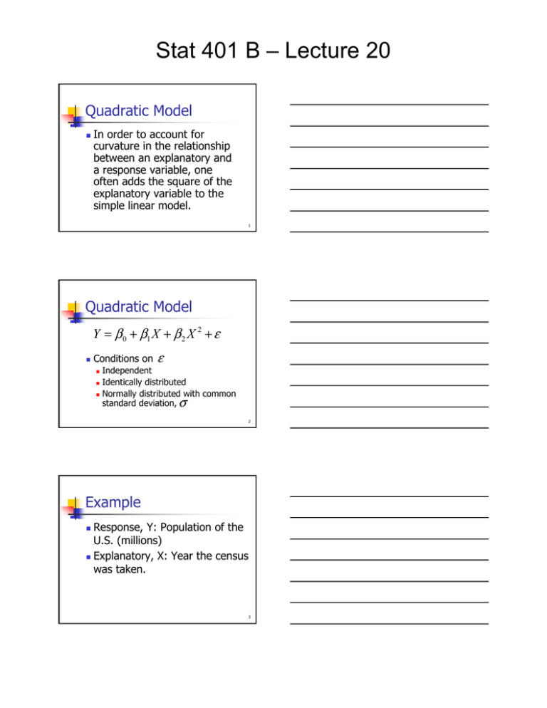
Stat 401 B – Lecture 20
Quadratic Model
„
In order to account for
curvature in the relationship
between an explanatory and
a response variable, one
often adds the square of the
explanatory variable to the
simple linear model.
1
Quadratic Model
Y = β 0 + β1 X + β 2 X 2 + ε
„
Conditions on
ε
Independent
„ Identically distributed
„ Normally distributed with common
standard deviation, σ
„
2
Example
Response, Y: Population of the
U.S. (millions)
„ Explanatory, X: Year the census
was taken.
„
3
Stat 401 B – Lecture 20
Quadratic Model
Predicted Population = 21006.1
–23.3785*Year + 0.00651*Year2
„ We cannot interpret the
estimated slope coefficients
because we cannot change Year
by 1 while holding Year2
constant.
„
4
Model Utility
F=8050.89, P-value<0.0001
„ The small P-value indicates
that the quadratic model
relating population to Year
and Year2 is statistically
significant (useful).
„
5
Statistical Significance
„
Year (added to Year2)
„
„
t=–33.48, P-value<0.0001
The P-value is small,
therefore the addition of
Year is statistically
significant.
6
Stat 401 B – Lecture 20
Statistical Significance
„
Year2 (added to Year)
„
„
t=35.22, P-value<0.0001
The P-value is small,
therefore the addition of
Year2 is statistically
significant.
7
Quadratic Model
R2=0.999 or 99.9% of the
variation in population can be
explained by the quadratic
model.
„ RMSE=2.77
„
8
Summary - Quadratic
The model is useful.
„ Each term is a statistically
significant addition.
„ 99.9% of the variation in
population is explained by the
quadratic model.
„
9
Stat 401 B – Lecture 20
Prediction
„
Year 2000
„
„
Predicted Population = 21006.1
– 23.3785(2000) +
0.0065063*(2000)2 = 274.3
million
Not bad as the actually figure
in 2000 was 281.422 million.
10
Prediction
„
Year 1800
„
„
Predicted Population = 21006.1
– 23.3785(1800) +
0.0065063*(1800)2 = 5.212
million
Very close to the actual value
of 5.308 million
11
250
Population
200
150
100
50
0
1750
1800
1850
1900
Year
1950
2000
12
Stat 401 B – Lecture 20
5.0
Residual
2.5
0.0
-2.5
-5.0
-7.5
1750
1800
1850
1900
Year
1950
2000
13
Plot of Residuals
The residuals wiggle around the
zero line. Hard to say whether
this is a pattern or not.
„ The residuals for 1940 and
1950 stick out. The quadratic
model over predicts for these
years.
„
14
Can we do better?
Could try higher order polynomial
terms like Year3 or Year4.
„ Year3 is not statistically significant
in a cubic model.
„ Year4 is not statistically significant
in a quartic model.
„
15
Stat 401 B – Lecture 20
Quadratic Model
There is still the issue of trying
to interpret the coefficients in
the quadratic model.
„ Again, creating a new
explanatory variable, Year2, has
introduced multicollinearity into
the quadratic model.
„
16
2000
1950
1900
Year
1850
1800
4000000
3900000
3800000
3700000
YearSqr
3600000
3500000
3400000
3300000
1800 1850 1900 1950 20003300000
36000003800000
17
Correlation
Year and Year2
„ Correlation: r = 0.9999
„ For the values that Year takes
on, there is an extremely strong
positive linear correlation with
Year2.
„
18
Stat 401 B – Lecture 20
Centering
Center Year by subtracting off
the mean before constructing
the squared term in the
quadratic model.
„ Mean year is 1890.
„
19
Quadratic Model
Predicted Population =
–2235.197 + 1.215*Year
+ 0.00651*(Year – 1890)2
„ Note that the estimated slope
for year is exactly the same as
in the simple linear model.
„
20
1950
1900
Year
1850
1800
10000
8000
6000
YearCtrSqr
4000
2000
0
-2000
1800
1850
1900
1950
-2000
2000 4000 6000 8000
21
Stat 401 B – Lecture 20
Correlation
Year and (Year – 1890)2
„ Correlation: r = –0.0000
„ For the values that Year takes
on, there is no linear correlation
with (Year – 1890)2.
„
22
Centering
„
Centering has completely
removed the multicollinearity
resulting from the inclusion of
the quadratic term in the
quadratic model.
23
Quadratic Model
Predicted Population = 61.926 +
1.215*(Year – 1890) +
0.00651*(Year – 1890)2
„ The predicted population in 1890
is 61.926 million.
„
24
Stat 401 B – Lecture 20
Quadratic Model
„
„
Predicted Population = 61.926 +
1.215*(Year – 1890) +
0.00651*(Year – 1890)2
For each additional year, the
population goes up, on average,
1.215 million.
25
Quadratic Model
„
„
Predicted Population = 61.926 +
1.215*(Year – 1890) +
0.00651*(Year – 1890)2
In addition to the average change
per year, there is a bigger
adjustment to this rate of change
the further away you are from 1890.
26
One Year Change
1880: Pred = 50.427 million
„ 1890: Pred = 61.926 million
„
„
Difference of 11.499
1980: Pred = 224.007
„ 1990: Pred = 248.526
„
„
Difference of 24.519
27