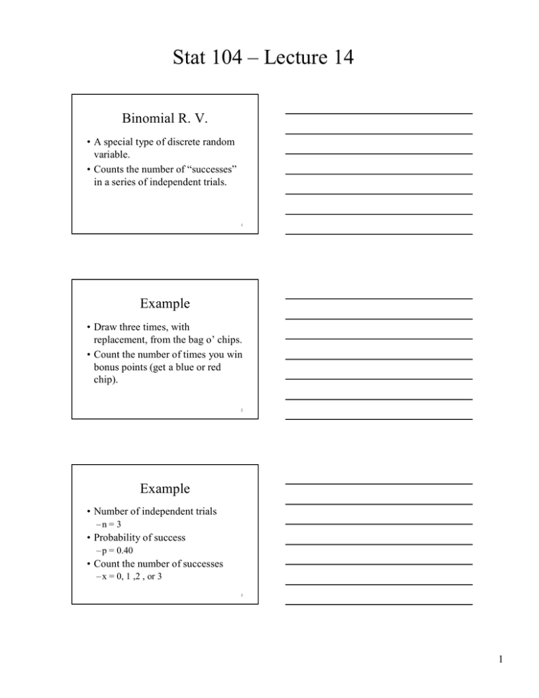
Stat 104 – Lecture 14
Binomial R. V.
• A special type of discrete random
variable.
• Counts the number of “successes”
in a series of independent trials.
1
Example
• Draw three times, with
replacement, from the bag o’ chips.
• Count the number of times you win
bonus points (get a blue or red
chip).
2
Example
• Number of independent trials
–n = 3
• Probability of success
– p = 0.40
• Count the number of successes
– x = 0, 1 ,2 , or 3
3
1
Stat 104 – Lecture 14
Tree Diagram
Trial 1
Trial 2
Trial 3
x
S
S
F
3
2
F
S
F
2
1
S
S
F
2
1
F
S
F
1
0
S
F
4
Probability Distribution
• P(3) = (0.4)*(0.4)*(0.4) = 0.064
• P(2) = (0.4)*(0.4)*(0.6) +
(0.4)*(0.6)*(0.4) +
(0.6)*(0.4)*(0.4)
= 3(0.4)2 (0.6) = 0.288
5
Probability Distribution
• P(1) = (0.4)*(0.6)*(0.6) +
(0.6)*(0.4)*(0.6) +
(0.6)*(0.6)*(0.4)
= 3(0.4)(0.6)2 = 0.432
• P(0) = (0.6)*(0.6)*(0.6) = 0.216
6
2
Stat 104 – Lecture 14
Binomial R. V.
X = number of times bonus points
are won on three draws from
the bag o’ chips.
x
0
P(x)
1
2
3
0.216 0.432 0.288 0.064
7
Binomial R. V.
• General formula for the probability
function.
n x

p
 x
P ( x ) = 
n

 

 x
=
(1 − p )n − x
x = 0 ,1,2 ,..., n
n!
x! (n − x )!
8
Example
• n = 3, p = 0.4, x = 2
 3


 2
P (2) = 
(0.4)2 (0.6 )3−2
3 ⋅ 2 ⋅1
(0.16)(0.6)
(2 ⋅ 1)(1)
P (2) = 0.288
=
9
3
Stat 104 – Lecture 14
Binomial R. V.
• Mean
µ = np
• Variance
σ 2 = np(1 − p )
10
Example
• n = 3, p = 0.40, (1 – p) = 0.60
• Mean
µ = np = 3(0.4 ) = 1.2
• Variance
σ 2 = np(1 − p )
= 3(0.4)(0.6 ) = 0.72
11
JMP
12
4
Stat 104 – Lecture 14
Another Example
• 38% (p =0.38) of people in the
United States have O+ blood type.
• If ten (n = 10) people come in to
donate blood, what is the chance
that 3 (x = 3) of them will have
O+?
13
Example
• n = 10, p = 0.38, x = 3
 10 


 3 
P (3 ) = 
(0.38)3 (0.62)7
10!
(0.054872)(0.035216146)
(3! )(7! )
P (3 ) = 0.2319
=
14
P(3) = 0.2319
15
5