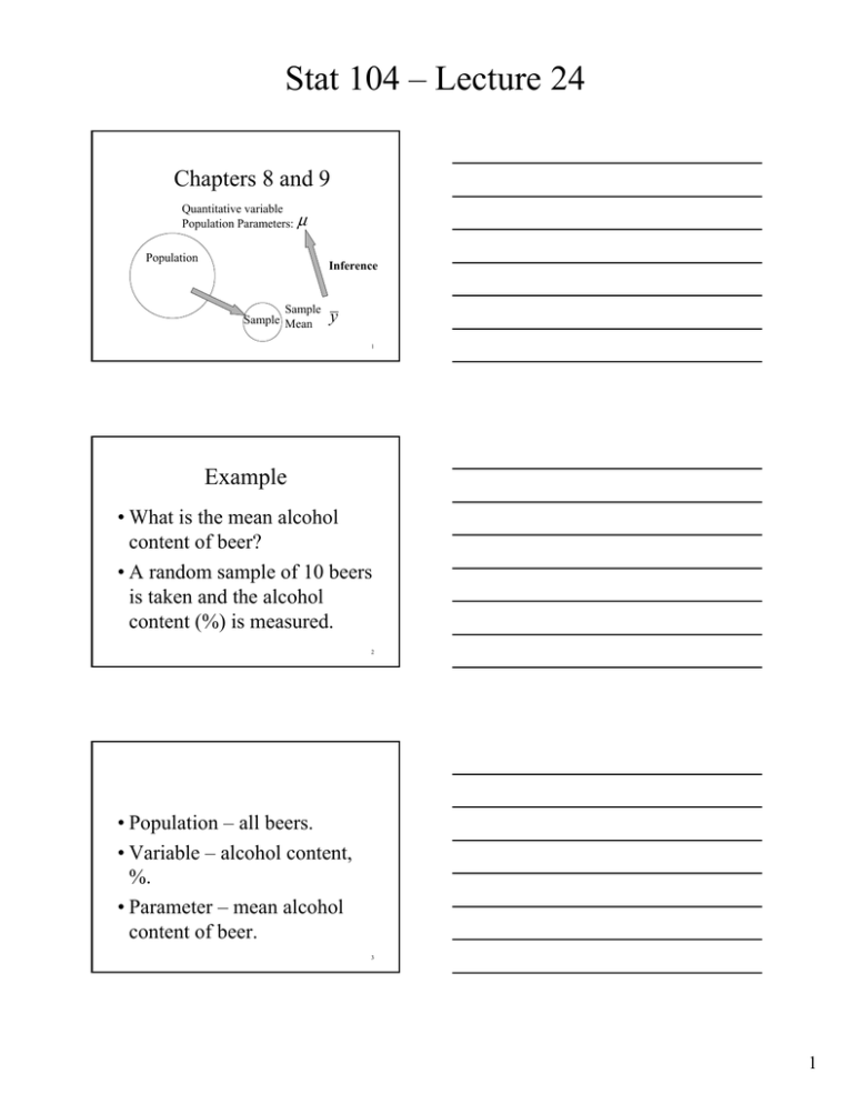
Stat 104 – Lecture 24
Chapters 8 and 9
Quantitative variable
Population Parameters: μ
Population
Inference
Sample
Sample Mean
y
1
Example
• What is the mean alcohol
content of beer?
• A random sample of 10 beers
is taken and the alcohol
content (%) is measured.
2
• Population – all beers.
• Variable – alcohol content,
%.
• Parameter – mean alcohol
content of beer.
3
1
Stat 104 – Lecture 24
Sample Data – Alcohol (%)
Molson
Canadian
Michelob
Dark
Big Barrel
Lager
Hamm’s
5.19
Tsingtao
4.79
4.76
4.32
4.53
Heineken
Dark
O’Keefe
Canadian
Olympia
Lager
Miller
Draft
Guinness
Stout
5.17
4.96
4.78
4.85
4.27
4
Sample Summary
• Sample size:
–n = 10
• Sample mean:
– y = 4.762
• Sample standard deviation:
–s = 0.314
5
Sampling Distribution of y
Quantitative variable
Population Parameters:μ , σ
Population
Sample Sample
Mean,
y
6
2
Stat 104 – Lecture 24
Summary
• Sampling from a population that
follows a Normal Model.
• Distribution of the sample mean, y
–Shape: Normal model
–Center: μ
σ
–Spread: SD( y ) =
n
7
Unknown, σ
• If we do not know the value
of the population standard
deviation we cannot
standardize and cannot use
table Z.
8
Unknown,σ
• We can use the sample
standard deviation, s, as an
estimate of the population
standard deviation, σ .
9
3
Stat 104 – Lecture 24
Unknown, σ
• We can NOT continue to use
the standard normal
distribution or Table Z.
• Why?
10
11
12
4
Stat 104 – Lecture 24
95% Confidence?
• Simulation illustrating
repeating the procedure.
• http://statweb.calpoly.edu/chance
/applets/ConfSim/ConfSim.html
13
14
Quantitative Variable
• Confidence Interval for μ .
⎛ s ⎞
⎛ s ⎞
y − t* ⎜
⎟ to y + t * ⎜
⎟
⎝ n⎠
⎝ n⎠
• t* found in Table T, df = n – 1
15
5
Stat 104 – Lecture 24
Quantitative variable
• Test statistic.
t=
y−μ
, Table T ⇒ P - value
⎛ s ⎞
⎜
⎟
⎝ n⎠
16
Confidence Interval for μ
⎛ s ⎞
⎛ s ⎞
y − t* ⎜
⎟ to y + t * ⎜
⎟
n
n
⎝
⎠
⎝
⎠
df = n − 1
17
Inference for μ
• Do NOT use Table Z!
Table Z
• Use Table T instead!
18
6