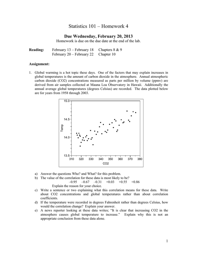
Statistics 101 – Homework 4
Due Wednesday, February 20, 2013
Homework is due on the due date at the end of the lab.
Reading:
February 13 – February 18
February 20 – February 22
Chapters 8 & 9
Chapter 10
Assignment:
1. Global warming is a hot topic these days. One of the factors that may explain increases in
global temperatures is the amount of carbon dioxide in the atmosphere. Annual atmospheric
carbon dioxide (CO2) concentrations measured as parts per million by volume (ppmv) are
derived from air samples collected at Mauna Loa Observatory in Hawaii. Additionally the
annual average global temperatures (degrees Celsius) are recorded. The data plotted below
are for years from 1958 through 2003.
15.0
Temp
14.5
14.0
13.5
310
320
330
350
340
CO2
360
370
380
a) Answer the questions Who? and What? for this problem.
b) The value of the correlation for these data is most likely to be?
–0.95 –0.67 –0.31 +0.03 +0.55 +0.86
Explain the reason for your choice.
c) Write a sentence or two explaining what this correlation means for these data. Write
about CO2 concentrations and global temperatures rather than about correlation
coefficients.
d) If the temperature were recorded in degrees Fahrenheit rather than degrees Celsius, how
would the correlation change? Explain your answer.
e) A news reporter looking at these data writes; “It is clear that increasing CO2 in the
atmosphere causes global temperature to increase.” Explain why this is not an
appropriate conclusion from these data alone.
1
2. The website www.realbeer.com gives calories, carbohydrates and alcohol content (% by
volume) for over 200 beers. A random sample of 10 beers was selected and the calories and
alcohol content (% by volume) of the beers in the sample are listed below.
Beer Name
Budweiser
Coors Original
Weinhard’s Amber Ale
Dundee Honey Brown
Keystone Light
Alcohol %
5.0
5.0
5.3
4.5
4.2
Calories
143.0
148.0
169.0
150.0
100.0
Beer Name
Kilarney's Red Lager
Michelob Amber Bock
Redhook ESB
Sierra Nevada Summerfest
Yuengling Porter
Alcohol %
5.0
5.2
5.8
4.9
4.5
Calories
197.0
166.0
179.0
158.0
152.5
a) Answer the questions Who? and What? for this problem.
b) Plot the data. Use Calories as the explanatory variable, x, and Alcohol % as the response,
y. Describe the relationship between Calories and Alcohol %.
c) Compute the mean and standard deviation for the Alcohol. Round final answers to 4
decimal places.
d) Compute the mean and standard deviation for the Calories. Round final answers to 4
decimal places.
e) Using ∑ ( x − x )( y − y ) = 73.8 , compute the correlation between Calories and Alcohol %.
f)
g)
h)
i)
j)
k)
Round final answer to 3 decimal places.
Compute the estimate of the slope for the least squares regression line. Round final
answer to 4 decimal places.
Give an interpretation of the estimated slope within the context of the problem.
Compute the estimate of the intercept for the least squares regression line. Round final
answer to 4 decimal places.
Give the equation of the least squares regression line. Use this equation to predict the
Alcohol % for a beer with 150 calories.
What is the residual for Dundee Honey Brown?
Give the value of R2 for this regression. Give an interpretation of this value within the
context of the problem.
3. The December 2003 issue of Kiplinger’s Personal Finance published data on the 2004 model
year cars and trucks. The weight (pounds) and EPA estimated highway mileage (mpg) for 57
cars are displayed below. The data, Fuel Economy Data, are on the main Stat 101 L course
page (www.public.iastate.edu/~wrstephe/stat101L.html) under Homework 4. Use JMP to
look at the distribution of Highway mpg and the relationship between Weight (explanatory,
x) and Highway mpg (response, y). Use the JMP output to help you answer the questions
below. Be sure to attach the JMP output to your assignment.
a) Describe the distribution of Highway mpg values. Make sure to include in your
description the five number summary, the mean and standard deviation, and the shape of
the histogram. Are there any outliers?
b) Describe the scatter plot of Highway mpg versus Weight. Give the regression equation
for predicting Highway mpg from Weight. Use the regression equation to predict the
Highway mpg for a car weighing 3000 pounds. Give an interpretation of the estimated
slope. Give the value of R2 and an interpretation of this value. Finally, describe the plot
of residuals versus weight values and make note of any potential problems with the
regression.
2