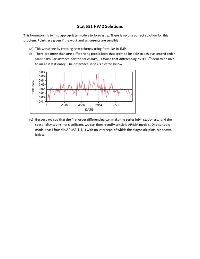
Stat 551 HW 2 Solutions This homework is to find appropriate models to forecast yt. There is no one correct solution for this problem. Points are given if the work and arguments are sensible. Difference
(a) This was done by creating new columns using formulas in JMP. (b) There are more than one differencing possibilities that seem to be able to achieve second order stationary. For instance, for the series ln(yt), I found that differencing by D1D 40 seem to be able to make it stationary. The difference series is plotted below. (c) Because we see that the first order differencing can make the series ln(yt) stationary, and the seasonality seems not significant, we can then identify sensible ARIMA models. One sensible model that I found is ARIMA(1,1,1) with no intercept, of which the diagnostic plots are shown below. Residuals
0.03
Residual Value
0.02
0.01
0.00
-0.01
-0.02
-0.03
0
2318
4636
6954
9272
DATE
Lag AutoCorr -.8-.6-.4-.2 0 .2 .4 .6 .8
1.0000
0
0.1287
1
0.0678
2
-0.0565
3
-0.0056
4
-0.2127
5
-0.0210
6
-0.0456
7
-0.1353
8
-0.0262
9
0.1399
10
0.1751
11
-0.0373
12
-0.0128
13
0.0078
14
-0.0724
15
0.1011
16
-0.0149
17
0.1382
18
-0.0825
19
0.0857
20
0.0378
21
0.0362
22
-0.1511
23
-0.0181
24
0.0673
25
Ljung-Box Q
.
2.1208
2.7133
3.1288
3.1329
9.1184
9.1769
9.4564
11.9407
12.0343
14.7360
19.0049
19.2001
19.2233
19.2320
19.9884
21.4761
21.5086
24.3426
25.3626
26.4727
26.6903
26.8920
30.4473
30.4985
31.2172
p-Value
.
0.1453
0.2575
0.3722
0.5358
0.1044
0.1639
0.2215
0.1539
0.2114
0.1420
0.0610
0.0838
0.1163
0.1563
0.1724
0.1609
0.2044
0.1441
0.1489
0.1508
0.1813
0.2154
0.1370
0.1688
0.1819
Lag
0
1
2
3
4
5
6
7
8
9
10
11
12
13
14
15
16
17
18
19
20
21
22
23
24
25
Partial -.8-.6-.4-.2 0 .2 .4 .6 .8
1.0000
0.1287
0.0521
-0.0729
0.0070
-0.2096
0.0297
-0.0228
-0.1631
0.0235
0.1181
0.1405
-0.1098
-0.0672
0.0515
-0.0466
0.1692
-0.0871
0.1840
-0.0577
0.0227
0.0716
-0.0509
-0.0567
0.0025
0.1508
(d) 95% prediction limits for my model from (c) for s=12 future values of yt. 8000
7000
6000
Y
5000
4000
3000
2000
1000
0
0
Y
2000 4000 6000 8000 1000012000
GNP predicted
DATE
Upper CL (0.95) GNP
(e) Fitting ARIMA(1,1,1) with no intercept model on the five contaminated series of ln(yt), we can get the following fitted parameters. 1. No contamination 2. Doubled at t=25 3. Doubled at t=50 4. Doubled at t=75 5. Doubled at t=100 6. Doubled at t=125 The above fitted parameters show that contamination has a serious effect on estimation of an AR parameter. If the contamination is near the end of a time series dataset , it will also have a serious effect on estimation of a MA parameter. However, if the contamination is not at the beginning or in the middle, it does not seem to have significant effect on estimation of a MA parameter. Compare forecasts s=4,8, 12 uncontaminated t=25 t=50 t=75 s=4 8.674735 8.573254 8.569558 8.567928
s=8 8.715713 8.573254 8.569558 8.567928
s=12 8.755691 8.573254 8.569558 8.567928
(f)
t=100 8.584568
8.584568
8.584568
t=125 11.34189 11.99709 12.15554 Fitting ARIMA(1,1,1) with no intercept model on the five contaminated series of ln(yt), we can get the following fitted parameters.
1. No contamination 2. Step change at t=25 3. Step change at t=50 4. Step change at t=75 5. Step change at t=100 6. Step change at t=125 Compare forecasts s=4,8,12 uncontaminated s=4 8.674735 s=8 8.715713 s=12 8.755691 t25 8.624948
8.624944
8.624944
t50 8.627008
8.627001
8.627001
t75 8.629923
8.629913
8.629913
t100 8.631565
8.631524
8.631522
t125 8.644293 8.653095 8.659797 (g) The fitted parameters for the transfer function model using a pulse at time t=100 covariate are: Output
The fitted and predicted values are shown in the graph below: The fitted parameters for the transfer function model using a level shift at time t=100 covariate are: The fitted and predicted values are shown in the graph below: Output
(h) The best model that I found is ARIMA(1,1,1) on ln(yt) with covariates first differenced log PCE and that of GPDI. The fitted parameters are as following. Residual Value
The residual plot is as following, which looks like white noise. (i) Comparing the two models, MAE is smaller for the model with covariates; MAPE is smaller for the model without covariates. Therefore, it is not clear which model is definitely better. Model Summary
DF
Sum of Squared Errors
Variance Estimate
Standard Deviation
Akaike's 'A' Information Criterion
Schwarz's Bayesian Criterion
RSquare
RSquare Adj
MAPE
MAE
-2LogLikelihood
121
0.00345407
0.0000125
0.00353565
-1047.4577
-1036.1445
0.88281475
0.87990933
35.880772
0.00284675
-957.32613
(j) and (k): the method of (j) is the same as (d); the method of (k) is the same as in (e) and (f).