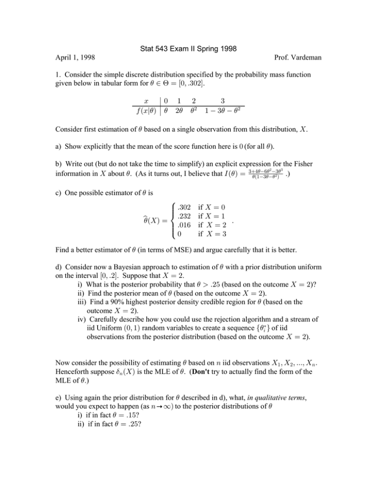
Stat 543 Exam II Spring 1998
April 1, 1998
Prof. Vardeman
1. Consider the simple discrete distribution specified by the probability mass function
given below in tabular form for ) − @ œ Ò!ß Þ$!#Ó.
B
0 ÐBl)Ñ
!
)
"
#)
#
)#
$
"  $)  ) #
Consider first estimation of ) based on a single observation from this distribution, \ .
a) Show explicitly that the mean of the score function here is ! (for all )).
b) Write out (but do not take the time to simplify) an explicit expression for the Fisher
)')# $)$
information in \ about ) . (As it turns out, I believe that MÐ)Ñ œ $%
)Ð"$))# Ñ .)
c) One possible estimator of ) is
Ú
Ý
Ý Þ$!#
s) Ð\Ñ œ Û Þ#$#
Ý
Ý Þ!"'
Ü!
if
if
if
if
\œ!
\œ"
.
\œ#
\œ$
Find a better estimator of ) (in terms of MSE) and argue carefully that it is better.
d) Consider now a Bayesian approach to estimation of ) with a prior distribution uniform
on the interval Ò!ß Þ#Ó. Suppose that \ œ #.
i) What is the posterior probability that )  Þ#& (based on the outcome \ œ #)?
ii) Find the posterior mean of ) (based on the outcome \ œ #).
iii) Find a 90% highest posterior density credible region for ) (based on the
outcome \ œ #).
iv) Carefully describe how you could use the rejection algorithm and a stream of
iid Uniform Ð!ß "Ñ random variables to create a sequence Ö)3‡ × of iid
observations from the posterior distribution (based on the outcome \ œ #).
Now consider the possibility of estimating ) based on 8 iid observations \" ß \# ß ÞÞÞß \8 Þ
Henceforth suppose $8 Ð\Ñ is the MLE of ) . (Don't try to actually find the form of the
MLE of ) .)
e) Using again the prior distribution for ) described in d), what, in qualitative terms,
would you expect to happen (as 8 p _Ñ to the posterior distributions of )
i) if in fact ) œ Þ"&?
ii) if in fact ) œ Þ#&?
The graph attached to this exam is for the loglikelihood in this problem, based on a
sample of 8 œ "!! observations with the frequency distribution below
B
frequency
!
19
"
$%
#
(
$
%!
f) Use the graph and give a large sample 90% confidence interval for ) based on the
large sample distribution of $8 Ð\Ñ and the observed (not expected) Fisher information in
this sample.
g) Use the graph of the loglikelihood j8 Ð)Ñ and give a large sample 90% confidence
interval for ) based on the large sample distribution of j8 Ð$8 Ð\ÑÑ  j8 Ð)Ñ.
2. Consider the problem of estimation in the Weibull family of distributions based on 8
iid observations \" ß \# ß ÞÞÞß \8 Þ For scale and location parameters ! and " , the
loglikelihood here is À
8
"
j8 Ð!ß " Ñ œ 8ln"  8" ln!  Ð"  "Ñ"lnB3   " "B3" 
!
3œ"
3œ"
8
and the likelihood equations reduce to
! lnB3 Ñ
Î ! B"3 lnB3
Ð 3œ"
Ó
3œ"
"œÐ

Ó
8
8
"
!
B
3
Ï
Ò
8
"
8
3œ"
and
!œ
Î
Ï
! B"3
3œ"
8
8
Ñ
Ò
"
"
.
There are no closed form solutions for these equations (i.e. there are no explicit formulas
for MLEs here). However, suppose that I want to make a 90% approximate confidence
interval for " (the shape parameter). Describe in as much detail as possible how you
would go about producing such an interval.