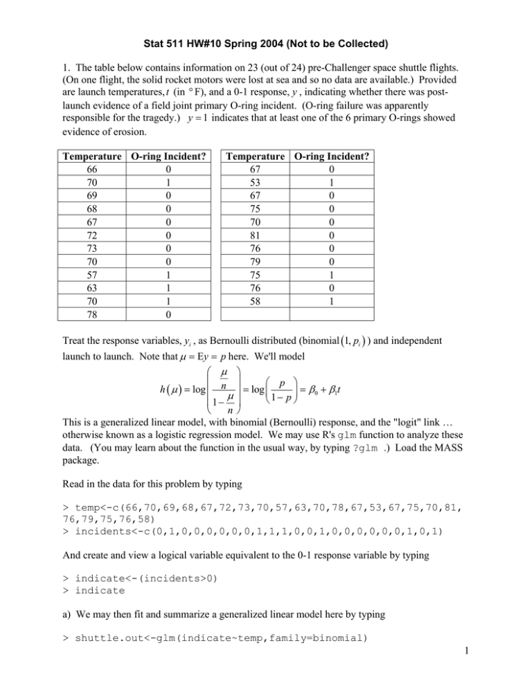
Stat 511 HW#10 Spring 2004 (Not to be Collected)
1. The table below contains information on 23 (out of 24) pre-Challenger space shuttle flights.
(On one flight, the solid rocket motors were lost at sea and so no data are available.) Provided
are launch temperatures, t (in ° F), and a 0-1 response, y , indicating whether there was postlaunch evidence of a field joint primary O-ring incident. (O-ring failure was apparently
responsible for the tragedy.) y = 1 indicates that at least one of the 6 primary O-rings showed
evidence of erosion.
Temperature O-ring Incident?
66
0
70
1
69
0
68
0
67
0
72
0
73
0
70
0
57
1
63
1
70
1
78
0
Temperature O-ring Incident?
67
0
53
1
67
0
75
0
70
0
81
0
76
0
79
0
75
1
76
0
58
1
Treat the response variables, yi , as Bernoulli distributed (binomial (1, pi ) ) and independent
launch to launch. Note that µ = Ey = p here. We'll model
 µ 


 p 
h ( µ ) = log  n  = log 
 = β 0 + β1t
µ
1− p 
1− 
n

This is a generalized linear model, with binomial (Bernoulli) response, and the "logit" link …
otherwise known as a logistic regression model. We may use R's glm function to analyze these
data. (You may learn about the function in the usual way, by typing ?glm .) Load the MASS
package.
Read in the data for this problem by typing
> temp<-c(66,70,69,68,67,72,73,70,57,63,70,78,67,53,67,75,70,81,
76,79,75,76,58)
> incidents<-c(0,1,0,0,0,0,0,0,1,1,1,0,0,1,0,0,0,0,0,0,1,0,1)
And create and view a logical variable equivalent to the 0-1 response variable by typing
> indicate<-(incidents>0)
> indicate
a) We may then fit and summarize a generalized linear model here by typing
> shuttle.out<-glm(indicate~temp,family=binomial)
1
> summary(shuttle.out)
The logit is the default link for binomial responses, so we don't need to specify that in the
function call.
Notice that the case β1 < 0 is the case where low temperature launches are more dangerous than
warm day launches. NASA managers ordered the launch after arguing that these and other data
data showed no relationship between temperature and O-ring failure. Was their claim correct?
Explain.
b) glm will provide estimated mean responses (and corresponding standard errors) for values of
the explanatory variable(s) in the original data set. To see estimated means
n
1
and corresponding standard errors, type
µli = l
pi =
1 + exp ( − β 0 − β1ti )
> shuttle.fits<-predict.glm(shuttle.out,type="response",
se.fit=TRUE)
> shuttle.fits$fit
> shuttle.fits$se.fit
Plot estimated means versus t . Connect those with line segments to get a rough plot of the
estimated relationship between t and p . Plot "2 standard error" bands around that response
function as a rough indication of the precision with which the relationship between t and p could
be known from the pre-Challenger data.
The temperature at Cape Canaveral for the last Challenger launch was 31 ° F. Of course, hindsight is always perfect, but what does your analysis here say might have been expected in terms
of O-ring performance at that temperature? You can get an estimated 31 ° F mean and
corresponding standard error by typing
> predict.glm(shuttle.out,data.frame(temp=31),se.fit=TRUE,
type="response")
2. An engineering student group worked with the ISU press on a project aimed at reducing jams
on a large collating machine. They ran the machine at 3 "Air Pressure" settings and 2 "Bar
Tightness" conditions and observed
y = the number of machine jams experienced in
k seconds of machine run time
(Run time does not include the machine "down" time required to fix the jams.) Their results are
below.
Air Pressure
1 (low)
2 (medium)
3 (high)
1
2
3
Bar Tightness
1 (tight)
1
1
2 (loose)
2
2
y , Jams
27
21
33
15
6
11
k , Run Time
295
416
308
474
540
498
2
Motivated perhaps by a model that says times between jams under a given machine set-up are
independent and exponentially distributed, we will consider an analysis of these data based on a
model that says the jam counts are independent Poisson variables. For
µ = the mean count at air pressure i and
bar tightness j
suppose that
Notice that this says
log µij = µ + α i + β j + log kij
(*)
µij = kij exp ( µ + α i + β j )
(If waiting times between jams are independent exponential random variables, the mean number
of jams in a period should be a multiple of the length of the period, hence the multiplication here
by kij is completely sensible.) Notice that equation (*) is a special case ( γ = 1 ) of the relationship
log µij = µ + α i + β j + γ log kij
which is in the form of a generalized linear model with link function h( µ ) = log ( µ ) . As it turns
out, glm will fit a relationship like (*) for a Poisson mean that includes an "offset" term ( log kij
here). Enter the data for this problem and set things up by typing
>
>
>
>
>
>
>
A<-c(1,2,3,1,2,3)
B<-c(1,1,1,2,2,2)
y<-c(27,21,33,15,6,11)
k<-c(295,416,308,474,540,498)
AA<-as.factor(A)
BB<-as.factor(B)
options(contrasts=c("contr.sum","contr.sum"))
a) Fit and view some summaries for the Poisson generalized linear model (with log link and
offset) by typing
> collator.out<-glm(y~AA+BB,family=poisson,offset=log(k))
> summary(collator.out)
The log link is the default for Poisson observations, so one doesn’t have to specify it in the
function call. Does it appear that there are statistically detectable Air Pressure and Bar Tightness
effects in these data? Explain. If one wants small numbers of jams, which levels of Air Pressure
and Bar Tightness does one want?
b) Notice that estimated "per second jam rates" are given by
exp ( µ + α i + β j )
Give estimates of all 6 of these rates based on the fitted model.
c) One can get R to find estimated means corresponding to the 6 combinations of Air Pressure
and Bar Tightness for the corresponding values of k . This can either be done on the scale of the
observations or on the log scale. To see these first of these, type
> collator.fits<-predict.glm(collator.out,type="response",
se.fit=TRUE)
> collator.fits$fit
> collator.fits$se
3
How are the "fitted values" related to your values from b)?
To see estimated/fitted log means and standard errors for those, type
> lcollator.fits<-predict.glm(collator.out,se.fit=TRUE)
> lcollator.fits$fit
> lcollator.fits$se
3. Do Problem 2 of the Spring 2003 Stat 511 Final Exam.
4