STAT 511
Solution to HW 1
Spring 2008
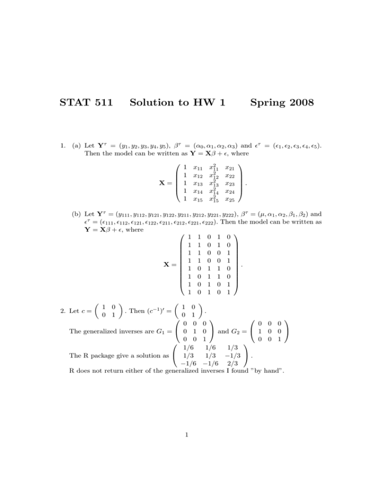
1. (a) Let Yτ = (y1 , y2 , y3 , y4 , y5 ), β τ = (α0 , α1 , α2 , α3 ) and ²τ = (²1 , ²2 , ²3 , ²4 , ²5 ).
Then the model can be written as Y = Xβ + ², where


1 x11 x211 x21
 1 x12 x212 x22 


2

X=
 1 x13 x13 x23  .
2

 1 x14 x
14 x24
2
1 x15 x15 x25
(b) Let Yτ = (y111 , y112 , y121 , y122 , y211 , y212 , y221 , y222 ), β τ = (µ, α1 , α2 , β1 , β2 ) and
²τ = (²111 , ²112 , ²121 , ²122 , ²211 , ²212 , ²221 , ²222 ). Then the model can be written as
Y = Xβ + ², where


1 1 0 1 0
 1 1 0 1 0 


 1 1 0 0 1 


 1 1 0 0 1 

.
X=

1
0
1
1
0


 1 0 1 1 0 


 1 0 1 0 1 
1 0 1 0 1
µ
¶
1 0
.
. Then
=
2. Let c =
0 1



0 0 0
0



0 1 0
1
The generalized inverses are G1 =
and G2 =
0 0 1
0


1/6
1/6
1/3
1/3 −1/3  .
The R package give a solution as  1/3
−1/6 −1/6 2/3
R does not return either of the generalized inverses I found ”by
1 0
0 1
¶
µ
(c−1 )0
1

0 0
0 0 
0 1
hand”.
3. The X matrix and M matrix are



1 1 0 0 0
.5 .5 0 0 0
0
0
 .5 .5 0 0 0
 1 1 0 0 0 
0
0



 0 0 1 0 0
 1 0 1 0 0 
0
0



 M = 0 0 0 1 0
0
0
1
0
0
1
0
X=



 0 0 0 0 1/3 1/3 1/3
 1 0 0 0 1 



 0 0 0 0 1/3 1/3 1/3
 1 0 0 0 1 
0 0 0 0 1/3 1/3 1/3
1 0 0 0 1





.




It is easy to verify that M = M 0 and M M = M. Thus we just need to show
that C(X) = C(M ). It is easy to see that the first two columns of M can be written as X(0, 0.5, 0, 0, 0)τ , the third and forth column of M is X(0, 0, 1, 0, 0)τ and
X(0, 0, 0, 1, 0)τ . The last three columns of M are X(0, 0, 0, 0, 1/3)τ .
Another way is to calculate the PX directly, since PX = X(X τ X)− X τ and we can
easily get the answer using R.
4.
a. The least squares estimate of EY is Ŷ = X(X τ X)− X τ Y .
Then Ŷ τ = [1.5, 1.5, 4, 6, 4, 4, 4] from R. One possible b is bτ1 = [0, 1.5, 4, 6, 4].
Another possible b is bτ2 = [1, 0.5, 3, 5, 3] such that Xb = Ŷ .
b. Use R to get Ŷ τ = [1.5, 1.5, 4, 6, 4, 4, 4], (Y − Ŷ )τ = [−0.5, −0.5, 0, 0, −1, 1, 0],
Ŷ 0 (Y − Ŷ ) = 0, Y 0 Y = 107, Ŷ 0 Ŷ = 104.5 and (Y − Ŷ )0 (Y − Ŷ ) = 2.5.
5. All these distributions can be found through the conditional distribution of some
elements of a vector with a multivariate normal distribution, conditional on the other
elements of the vector and the linear combination of normal distribution random
variables.
a. The marginal distribution of y3 is N (0, 3).
b. The marginal joint distribution of y1 and y3 is MVN2
µµ
2
0
¶ µ
¶¶
4 2
,
.
2 3
c. y3 |y1 = 2 ∼ N (0, 2).
d. y3 |y1 = 2, y2 = −1 ∼ N (−1.5, 1).
¶¶
¶
µµ
¶ µ
µ
4 2
2
y1
.
,
|y2 = −1 ∼ MVN2
e.
2 2
−1.5
y3
√
f. ρ12 = 0, ρ13 = ρ23 = 1/ 3.
g. The distribution of u and v can be treat as


µµ ¶ µ
¶¶
µ ¶ µ
¶ y1
µ ¶
0
11 16
u
1 −1 1 
0

y2
,
.
=
+
∼ MVN2
9
16 40
v
3 1 0
1
y3
2
6. Using the function eigen() to obtain eigenvalues and eigenvectors of a matrix V,
we are able to compute its inverse square root, W = V −1/2 = U D−1/2 U 0 , where U
is the eigenvector matrix and D is the diagonal matrix of eigenvalues. Note that
W W = V −1 . From R, we get


0.6140 0.0564 −0.0931
W =  0.0564 0.4646 0.0564  .
−0.0931 0.0564 0.6140
7. Form the calculation of R, we have
µ
¶
−4002000 4001000
−1
A =
4001000 −4000000
8. We know that

P
X0


=


µ
B
−1
=
1334000 −1333667
−1333667 1333333
¶
.

0.8
0.2
0.2
0.2
0.2
0.2
0.8 −0.2 −0.2 −0.2 

0.2 −0.2
0.8 −0.2 −0.2 

0.2 −0.2 −0.2
0.8 −0.2 
0.2 −0.2 −0.2 −0.2
0.8
To show c ∈ C(X 0 ), it is enough to show that PX 0 c = c. So µ+τ1 , 2µ+τ1 +τ2 , τ1 −τ2
and (τ1 −τ2 )−(τ3 −τ4 ) are estimable. The c0 (X 0 X)− X 0 for these estimable parameters
are [0.5, 0.5, 0, 0, 0, 0, 0], [0.5, 0.5, 1, 0, 0, 0, 0], [0.5, 0.5, −1, 0, 0, 0, 0], [0.5, 0.5, −1, −1, 1/3, 1/3, 1/3]
respectively.
9. The R function is
library{MASS}
Project<-function(X) {
Px<-X%*%ginv(t(X)%*%X)%*%t(X)
return(Px)}
The function works well for X and X 0 in problem 3.
10.
a. Because

PX 0





1
= 
9





4
2
2
2
2
2
4 −2
1
1
2 −2
4
1
1
2
1
1
4 −2
2
1
1 −2
4
1
2 −1
2 −1
1
2 −1 −1
2
1 −1
2
2 −1
1 −1
2 −1
2
1
2
−1
2
−1
4
−2
−2
1
1
2
−1
−1
2
−2
4
1
−2
1
−1
2
2
−1
−2
1
4
−2
1
−1
2
−1
2
1
−2
−2
4







,






we found µ+α1 +β1 +αβ11 and (αβ12 −αβ11 )−(αβ22 −αβ21 ) are estimable. The
c0 (X 0 X)− X 0 are [0.5, 0.5, 0, 0, 0, 0, 0, 0] and [−0.5, −0.5, 0.5, 0.5, 0.5, 0.5, −0.5, −0.5].
3
b. It is not testable. The first row of C is not in C(X 0 ).
11. The hypothesis can be written as
H0 : (0, x11 − x12 , x211 − x212 , x21 − x22 )(α0 , α1 , α2 , α3 )τ = 0.
So here C = (0, x11 − x12 , x211 − x212 , x21 − x22 ), β = (α0 , α1 , α2 , α3 )τ and d = 0.
4