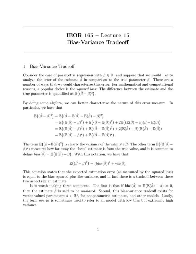
IEOR 165 – Lecture 15
Bias-Variance Tradeoff
1 Bias-Variance Tradeoff
Consider the case of parametric regression with β ∈ R, and suppose that we would like to
analyze the error of the estimate β̂ in comparison to the true parameter β. There are a
number of ways that we could characterize this error. For mathematical and computational
reasons, a popular choice is the squared
loss:
(
) The difference between the estimate and the
2
true parameter is quantified as E (β̂ − β) .
By doing some algebra, we can better characterize the nature of this error measure. In
particular, we have that
(
)
(
)
E (β̂ − β)2 = E (β̂ − E(β̂) + E(β̂) − β)2
(
)
(
)
(
)
= E (E(β̂) − β)2 + E (β̂ − E(β̂))2 + 2E (E(β̂) − β)(β̂ − E(β̂)
(
)
(
)
(
= E (E(β̂) − β)2 + E (β̂ − E(β̂))2 + 2(E(β̂) − β)(E β̂) − E(β̂))
(
)
(
)
= E (E(β̂) − β)2 + E (β̂ − E(β̂))2 .
(
)
(
The) term E (β̂ −E(β̂))2 is clearly the variance of the estimate β̂. The other term E (E(β̂)−
β)2 measures how far away the “best” estimate is from the true value, and it is common to
(
)
define bias(β̂) = E E(β̂) − β . With this notation, we have that
(
)
E (β̂ − β)2 = (bias(β̂))2 + var(β̂).
This equation states that the expected estimation error (as measured by the squared loss)
is equal to the bias-squared plus the variance, and in fact there is a tradeoff between these
two aspects in an estimate.
(
)
It is worth making three comments. The first is that if bias(β̂) = E E(β̂) − β = 0,
then the estimate β̂ is said to be unbiased. Second, this bias-variance tradeoff exists for
vector-valued parameters β ∈ Rp , for nonparametric estimates, and other models. Lastly,
the term overfit is sometimes used to refer to an model with low bias but extremely high
variance.
1
2 Example: Estimating Variance
Suppose Xi ∼ N (µ, σ 2 ) for i = 1, . . . , n are iid random variables, where µ, σ 2 are both
unknown. Recall that we have considered two estimators for the variance
n
1 ∑
2
s =
(Xi − X)2
n − 1 i=1
1∑
σˆ2 =
(Xi − X)2 =
n i=1
n
n−1 2
s.
n
And recall that in the homework, we showed that
E(s2 ) = σ 2
E(σˆ2 ) = n−1 σ 2 .
n
2
In this example, we would say that s is an unbiased estimate of the variance because
(
)
(
)
bias(s2 ) = E E(s2 ) − σ 2 = E σ 2 − σ 2 = 0.
However, the σˆ2 is not an unbiased estimate of the variance because
(
)
(
)
bias(σˆ2 ) = E E(σˆ2 ) − σ 2 = E n−1 σ 2 − σ 2 = σ 2 /n.
n
It is tempting to say that s2 is a better estimate of the variance than σˆ2 becuase the former
is unbiased and the later is biased. However, lets examine the situation more closely. In
particular, suppose we compute the variance of both estimators. From the part of the course
on null hypothesis testing, we know that s2 ∼ σ 2 χ2 (n − 1)/n − 1, where χ2 (n − 1) denotes a
χ2 distribution with (n − 1) degrees of freedom. The variance of a χ2 (n − 1) distribution is
2(n − 1) by properties of the χ2 distribution. Hence, by properties of variance, we have that
var(s2 ) = 2σ 4 /(n − 1)
4
var(σˆ2 ) = 2 n−1
2 σ .
n
Since n > (n − 1) , dividing by (n − 1)n gives the inequality that 1/(n − 1) > (n − 1)/n2 .
This means that var(s2 ) > var(σˆ2 ): In words, the variance of σˆ2 is lower than the variance
of s2 .
2
2
2
Given that one estimate has lower bias and higher variance than the other, the natural
question to ask is which estimate has lower estimation error? Using the bias-variance tradeoff
equation, we have
E((s2 − σ 2 )2 ) = (bias(s2 ))2 + var(s2 ) = 02 + 2σ 4 /(n − 1) = 2σ 4 /(n − 1)
4
E((σˆ2 − σ 2 )2 ) = (bias(σˆ2 ))2 + var(σˆ2 ) = nσ2 + 2 n−1
σ 4 = 2n−1
σ 4 = (2n−1)(n−1)
· 2σ 4 /(n − 1).
n2
n2
2n2
But note that (2n − 1)(n − 1) < 2(n − 1)(n − 1) < 2n2 . As a result, (2n−1)(n−1)
< 1. This
2n2
means that
E((σˆ2 − σ 2 )2 ) ≤ E((s2 − σ 2 )2 ),
and so σˆ2 has lower estimation error than s2 when measuring error with the squared loss.
2
3 Stein’s Paradox
The situation of estimating variance for a Gaussian where a biased estimator has less estimation error than an unbiased estimator is not an exceptional case. Rather, the general
situation is that biased estimators have lower estimation errors. Such a conclusion holds in
even surprising cases such as the one described below.
Suppose we have jointly independent Xi ∼ N (µi , 1) for i = 1, . . . , n, with µi ̸= µj for i ̸= j.
This is a model where we have n measurements from Gaussians, where the mean of each
measurement is different. It is worth emphasizing that in this model we only have one
measurement from each different Gaussian. Now for this model, it is natural to consider
the problem of estimating the mean of each Gaussian. And the obvious choice is to use the
estimator
[
]′
µ̂ = X1 X2 . . . Xn .
This is an obvious choice because
[
]′
E(µ̂) = µ1 µ2 . . . µn .
It is hard to imagine that any other estimator could do better (in terms of estimation error)
than this estimator, because (i) we only have one data point for each Gaussian, and (ii) each
Gaussian is jointly independent.
However, this is the exact conclusion from Stein’s paradox. It turns out that if n ≥ 3, then
the following James-Stein estimator
(
n − 2)
µ̂JS = 1 −
· µ̂,
∥µ̂∥22
where µ̂ is as defined above, has strictly lower estimation error under the squared loss than
that of µ̂. This is paradoxical because the estimation of the means of Gaussians can be
impacted by the number of total Gaussians, even when the Gaussians are jointly independent.
The intuition is that as we try to jointly estimate more means, we can reduce the estimation
error by purposely adding some bias to the estimate. In this case, we bias the estimates
of the means towards zero. (This is sometimes called shrinkage in statistics, because we
are shrinking the values towards zero.) The error introduced by biasing the estimate is
compensated by a greater reduction in the variance of the estimate.
4 Proportional Shrinkage for OLS
Given that it can be the case that adding some bias can improve the estimation error, it is
interesting to consider how we can bias OLS estimates. Recall that the OLS estimate with
data (xi , yi ) for xi ∈ Rp , yi ∈ R, i = 1, . . . , n is given by
β̂ = arg min ∥Y − Xβ∥22 ,
3
where the matrix X ∈ Rn×p and the vector Y ∈ Rn are such that the i-th row of X is x′i
and the i-th row of Y is yi . One popular approach to adding shrinkage to OLS is known as
Ridge Regression, Tikhonov regularization, or L2-regularization. It is given by the solution
to the following optimization problem
β̂ = arg min ∥Y − Xβ∥22 + λ∥β∥22 ,
where λ ≥ 0 is a tuning parameter. (We will return to the question of how to choose the
value of λ in a future lecture.)
To understand why this method adds statistical shrinkage, consider the one-dimensional
special case where xi ∈ R. In this case, the estimate is given by
n
∑
β̂ = arg min
(yi − xi · β)2 + λβ 2
i=1
= arg min
=
n
∑
yi2 − 2yi xi β + x2i β 2 + λβ 2
i=1
∑
arg min( ni=1
−2yi xi )β + (λ +
∑n
i=1
x2i )β 2 +
∑n
i=1
yi2
Next, setting the derivative of the objective equal to zero gives
∑
∑
∑
∑
dJ
= ( ni=1 −2yi xi ) + 2(λ + ni=1 x2i )β = 0 ⇒ β̂ = ( ni=1 yi xi )/(λ + ni=1 x2i ).
dβ
When λ = 0, this is simply the OLS estimate. If λ > 0, then the denominator of the estimate
is larger; hence, the estimate will have a smaller absolute value (i.e., it will shrink towards
zero). If we can choose a good value of λ, then the estimate will have lower estimation error.
We will consider how to choose the value of λ in a future lecture.
4